![]()
![]()
![]()
This appendix introduces concepts of linear algebra needed in the mixed model framework. The material in this appendix is from Neter et al. (1990), Searle (1971, 1982, 1987) and Searle et al. (1992).
C.2 Matrix addition and multiplication
C.4 Linear (in)dependence and rank of matrix
C.7 Some basic theorems for matrices
C.8 Random vectors and matrices
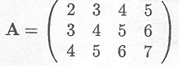
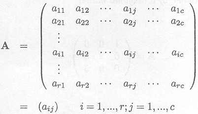
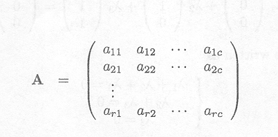
A matrix is a rectangular scheme of numbers, e.g.,
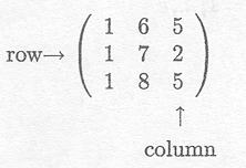
The general notation is
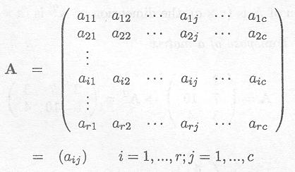
r is the number of rows
c is the number of columns
aij is the (i, j) entry or element of the matrix A.
The dimension of A is (r x c).
A matrix with c = 1 is called a column vector or vector, e.g.,

A matrix with r = 1 is called a row vector, e.g.,
The transpose of A (written AT) is obtained by interchanging rows and columns
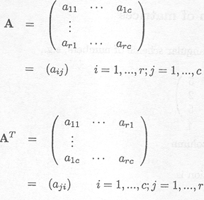
If the dimension of A is (r x c), the dimension of AT is (c x r).
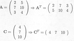
Example C.1.1 Transpose of a matrix
Find the (r x c) = (3 x 4) matrix for which aij = i + j
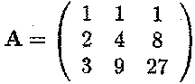
Find the (r x c) = (3 x 3) matrix for which aij = ij
Note: r = c then A is a square matrix.
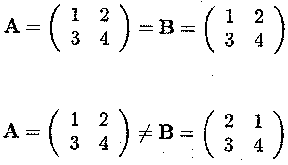
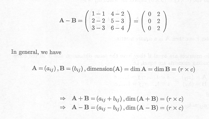
Two matrices are equal if they have the same dimension and if all the corresponding elements are equal, i.e.,
A = (aij) i = 1, ..., r; j = 1, ..., c
B = (bij ) i = 1, ..., r; j = 1, ..., c
and
aij = bij
Example C.1.2 Equality of matrices
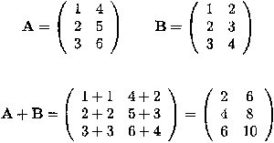
Adding (or subtracting) two matrices requires that they have the same dimension. The sum (difference) of two such matrices is another matrix whose elements consist of the sum (difference) of the corresponding elements of the two matrices.
Example C.2.1 Adding and subtracting matrices
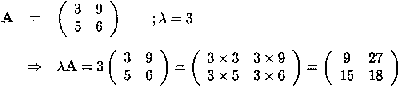
A matrix can be multiplied by a scalar or another matrix.
Multiplying a matrix with a scalar corresponds to multiplying each entry in the matrix by the scalar
![]()
Example C.2.2 Multiplying a matrix by a scalar
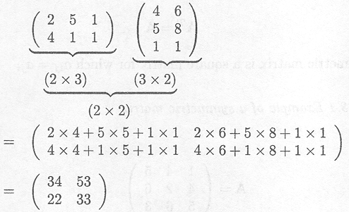
Multiplying a matrix A with another matrix B, leading to the product AB is only possible if the number of columns of the first matrix is equal to the number of rows of the second matrix, otherwise the product is undefined.
Assume that dim A = (r x c), then B must have c rows. If dim B = (c x s), the dimension of the product of the two matrices equals dim(AB) = (r x s) and the (i, j ) entry of AB is given by

Example C.2.3 Multiplying a matrix by another matrix
A different type of product of two matrices A and B is the Kronecker or direct product
A ![]() B. As compared to the product of matrices described above, the direct product exists for any two matrices. If
A is a (r x c) matrix given by
B. As compared to the product of matrices described above, the direct product exists for any two matrices. If
A is a (r x c) matrix given by
and B is a (p x q) matrix then the Kronecker or direct product A
![]() B is given by
B is given by
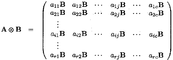
The resulting matrix A ![]() B is a (rp x cq) matrix.
B is a (rp x cq) matrix.
A symmetric matrix is characterised by
Thus a symmetric matrix is a square matrix for which aij = aji
Example C: 3.l Example of a symmetric matrix
A matrix is diagonal if it is a square matrix and if all off-diagonal elements are zero, thus aij = 0 if i # j
Example C.3.2 Example of a diagonal matrix
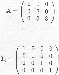
This matrix is caned the identity matrix with dimension 4.
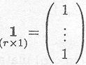
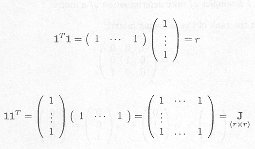
A vector with all entries unity is noted as
A square matrix with all entries unity is noted as
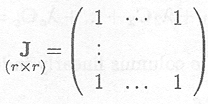
Example C.3.3 Examples of matrices with all entries unity
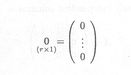
Finally, a zero vector has all entries equal to 0
A matrix
can also be written as a collection of column vectors
C = (C1 C2 ... Cc)
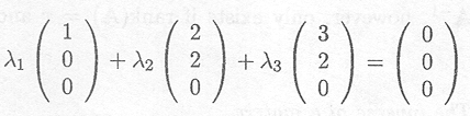
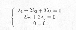
If ![]() 1C1 + +
1C1 + +![]() 2C2 + ... +
2C2 + ... + ![]() Cc = 0
Cc = 0
holds, we then call the set of c columns linearly independent.
We then say that rank(A) = c.
In general the rank(A) is the maximum number of linearly independent columns in the matrix A.
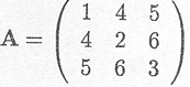
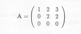
Example C.4.1 Examples of rank determination of a matrix
We determine the rank of the following matrix
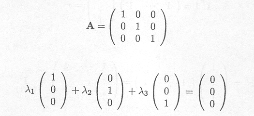
only holds if ![]() 1 = 2 = 3 = 0, and thus
rank(A) = 3.
1 = 2 = 3 = 0, and thus
rank(A) = 3.
Another matrix with linearly independent columns is
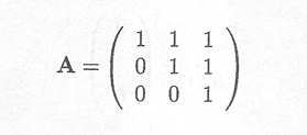
Indeed, the solution of set of equations
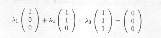
which can also be written as
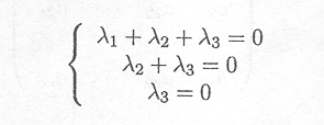
is easily seen to be ![]() l =
l = ![]() 2 =
2 = ![]() 3 = 0
3 = 0
Therefore, rank(A) = 3.
Finally, a matrix with linearly dependent columns is
The set of equations to be solved is
or equivalently
A solution (among an infinite number of solutions) is given by ![]() l =
l = ![]() 2 = 1,
2 = 1, ![]() 3 = .1. Thus, these columns are not linearly independent, and the rank is lower than 3, the number of columns.
3 = .1. Thus, these columns are not linearly independent, and the rank is lower than 3, the number of columns.
The three column vectors only span a two-dimensional space. The third column can be obtained by adding the first two columns. Therefore, the three vectors are not linearly independent.
The determinant ![]() A
A![]() is a polynomial of the elements of the square matrix
A, and thus a scalar value. It is the sum of certain products of elements of the matrix
A. The determinant only exists for square matrices.
is a polynomial of the elements of the square matrix
A, and thus a scalar value. It is the sum of certain products of elements of the matrix
A. The determinant only exists for square matrices.
Different methods exist to derive the determinant, and it quickly becomes cumbersome for matrices with high dimension.
The determinant of a scalar is the scalar itself. The determinant of a 2 x 2 matrix A
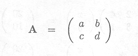
is given by
![]() A
A![]() = ad . bc
= ad . bc
The derivation of the determinant for matrices with higher dimensions is given by Searle (1982).
Let A be an (r x r) matrix (square matrix). The inverse of A is an (r x r) matrix denoted by A-1, such that
A-1A = AA-1 = Ir
Such a matrix A-1, however, only exists if rank(A) = r and this inverse is unique.
Example C.6.1 The inverse of a matrix
The inverse of
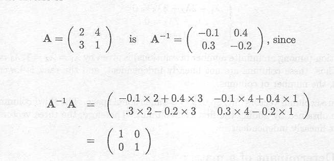
and also AA-1 = I2
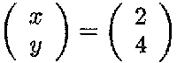
The inverse can be used to solve a set of equations such as

This can be written in matrix notation as
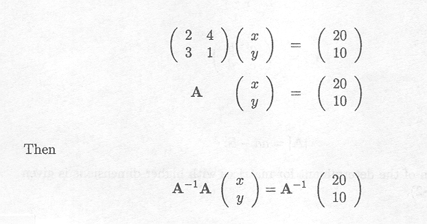
or
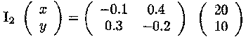
This yields
A continuous random variable Y is characterised by a specific density function fY (y), for instance the normal distribution. From the density one can calculate the probability that an observation takes its value in a specific range.
Furthermore, a random variable has an expected value E(Y) and a variance Var(Y), given by

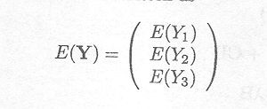
A vector consisting of three random variables Yl, Y2, Y3 can be written as
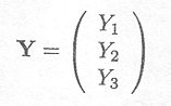
The expected value of this vector is written as
The variance-covariance matrix or dispersion matrix of the vector Y, written as D(Y) ![]() V equals
V equals
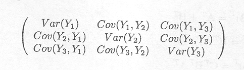
This matrix is symmetric.
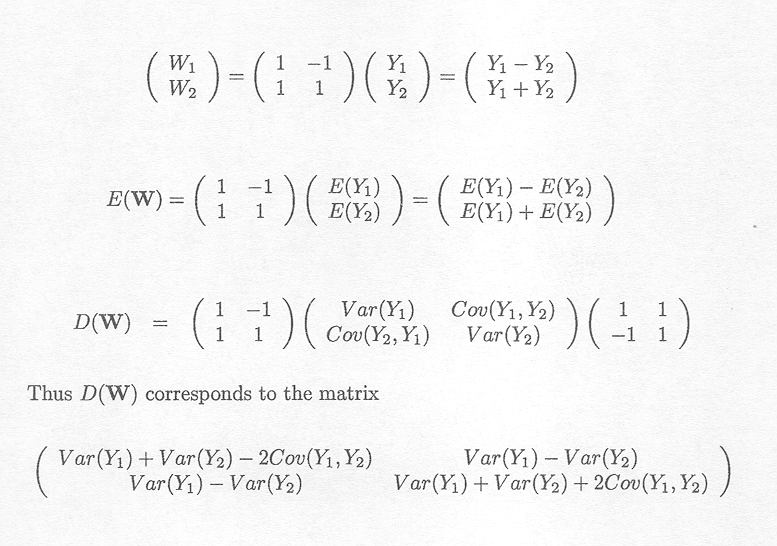
We typically encounter a random vector W which is obtained by premultiplying the random vector Y by a constant matrix A, i.e.,
Example C.8.1 Example of random vectors and matrices
![]()
![]()
![]()