The univariate normal density function is given by

for -![]() < x <
+
< x <
+![]() where µ is the mean and
where µ is the mean and![]() 2 > 0 is the variance ( is the standard deviation).
2 > 0 is the variance ( is the standard deviation).
This density is also called the Gaussian density and different examples of this family of densities with varying values of µ and
![]() are depicted in Figure D.1.
are depicted in Figure D.1.
The bivariate normal density function is given by
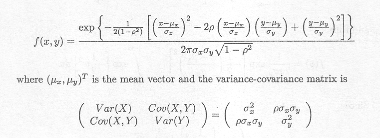
The constraints are![]()
![]() > 0,
> 0,![]()
![]() > 0 and —1 < p < 1. The parameter is the correlation coefficient.
> 0 and —1 < p < 1. The parameter is the correlation coefficient.
Examples of this family of densities with varying values of and µx = 0, µy = 0, ![]()
![]() = 1,
= 1,![]()
![]() = 1 are depicted in Figure D.2.
= 1 are depicted in Figure D.2.
Given f (x, y) the marginal density function f (y) is defined as
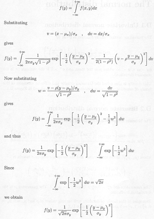
The marginal density f (y) is a normal density with mean µy and variance
![]()
![]() .
.
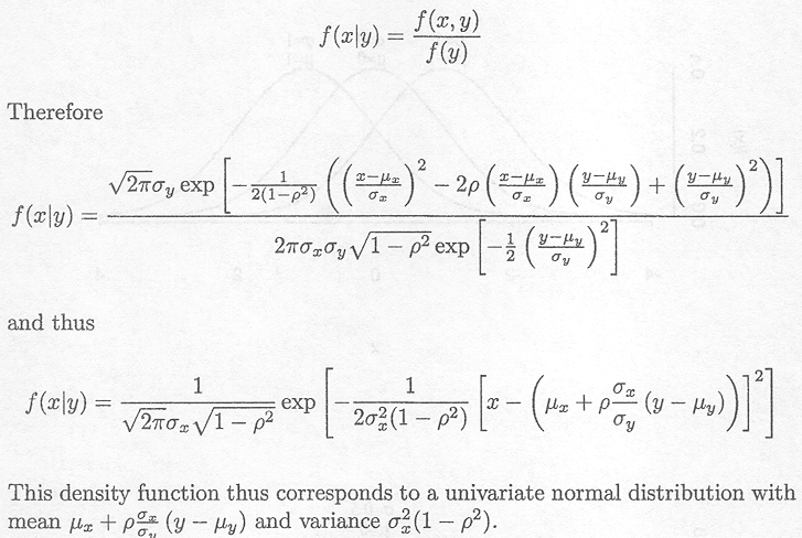
The conditional density f (x|y) is defined as
D.3 p-variate normal distribution
The p-variate normal density function is given by

where xT = (xl , .., xp), µT = {µl, ..., µp) and V is a full rank variance-covariance matrix.
V–1 is the inverse of V, V is the determinant of V.
Note that for p=2 we get the bivariate normal density.
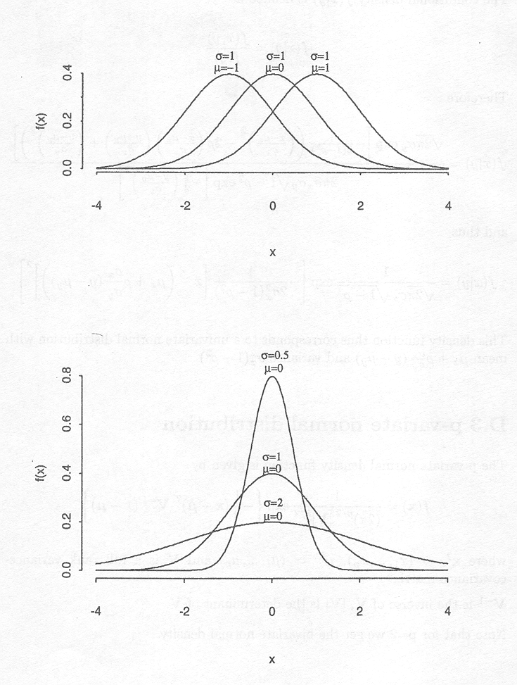
Figure D.1 Examples of the family of univariate normal densities. In the upper figure, three distributions are depicted with standard deviation equal to 1 and mean equal to –1, 0, 1. In the lower figure, the means of the three distributions are equal to 0 and the standard deviations are equal to 0.5, 1 and 2, respectively.
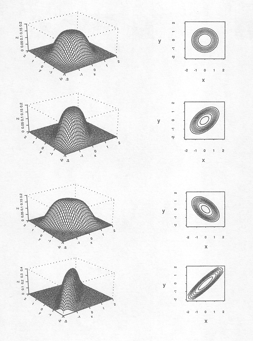
Figure D.2 Examples of the family of bivariate normal densities with µx = µy = 0;
![]()
![]() =
= ![]()
![]() = 1 and p = 0, 0.5, —0.5, 0.9 respectively.
= 1 and p = 0, 0.5, —0.5, 0.9 respectively.