2.2.1 The fixed effects model with one independent variable: one-way ANOVA
2.2.2 The fixed effects model with two independent variables: two-way ANOVA
2.3 A general description of the mixed model
2.3.1 The mixed model description based on individual observations
2.4 Variance component estimation and blup
2.4.1 Defining variance components
2.5 Statistical inference for fixed effects
2.5.1 Estimation of fixed effects and their variance
2.5.2 Estimation of linear combinations of fixed effects and their variance
In this chapter the theoretical basis of the mixed model is explained. The fixed effects model is first introduced in Section 2.2 so that it can be compared in subsequent sections with the mixed model. The analysis of data in the fixed effects model framework is demonstrated with one independent variable (one-way ANOVA) and with two independent variables (two-way ANOVA) . Two alternative models, the 'cell means model' and the 'overparameterised model' are described. It is further explained how particular hypotheses can be tested and specific linear combinations of parameters can be estimated in the framework of the two different models. Next, the problems that may occur when using the fixed effects model for the analysis of data which also contain random effects factors are studied.
Good textbooks on the analysis of linear models, and in specific fixed effects models, include Neter et al. (1990) and Hocking (1996). A more theoretical approach, with the emphasis on the linear algebraic model formulation, is given by Searle (1971, 1987).
In Section 2.3 a general description of the mixed model is given. The different data structures of the examples included in Chapter 1 are described in the mixed model framework.
In Section 2.4 it is shown how variance components, which correspond to the variation associated with the random effects factor, can be estimated in the mixed model framework by restricted maximum likelihood (REML), and how the individual effect of a level of a random effects factor can be predicted by the method of best linear unbiased prediction (BLUP).
In Section 2.5 estimation of fixed effects parameters and linear combinations thereof is explained and the distributional assumptions of these estimates are derived and used to obtain confidence intervals.
In Section 2.6, it is shown how hypotheses of interest can be tested in the mixed model framework.
There are two alternative formulations for the fixed effects model, the cell means model and the overparameterised model. As the statistical theory for the cell means model is easier, we explain this model first. Most statistical packages, however, use the overparameterised model, and this will be introduced after describing the cell means model.
The cell means model for a fixed effects model with one independent variable with a levels and nk observation per level k is given by
Ykl = µk + ekl, k = 1, ..., a; l = 1, ..., nk
where µk represents the kth individual cell mean, and the different cells represent different treatments.
The extensive way to write this model is
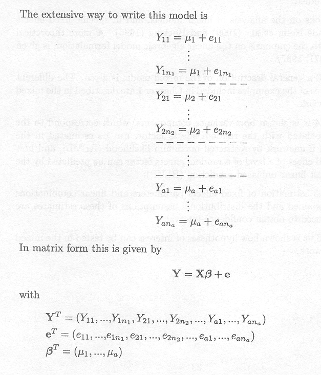
and
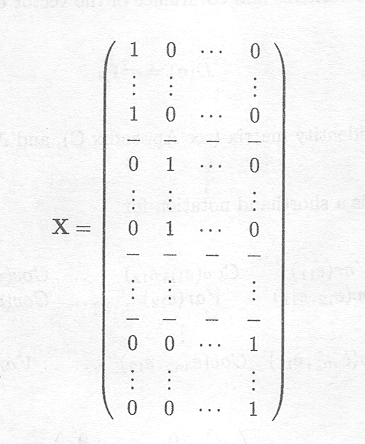
X is called the design matrix; the zero and one entries are called dummy variables.
We further require the classical ANOVA assumptions, i.e., the random error variables eij are independent with distribution N(0, s2).
Under these assumptions we have
E (ei j ) = 0
Var (eij) = s2 (homoscedasticity)

The expected value of the vector e can be rewritten in matrix notation as
E(e) = 0
This expression is a shorthand notation for
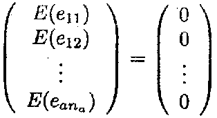
Furthermore, the variance and covariance of the vector e can be rewritten as
D(e) = s2IN
where IN, is the identity matrix (see Appendix C), and 
This expression is a shorthand notation for
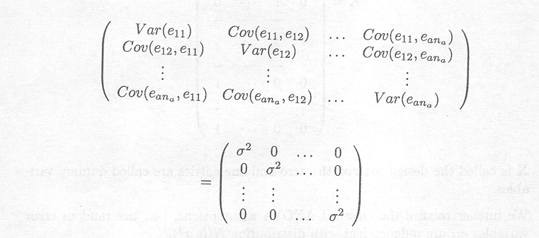
D(e) is an (N x N) matrix. E(e) is called the mean vector of the random vector e; D(e) is called the dispersion matrix or variance-covariance matrix of the random vector e.
A short way to write that the random errors eij are independent with distribution N(0,s2) is
e ~ MVN(0, s2IN)
In words: the random vector e is multivariate normal with zero as mean vector and the diagonal matrix s2IN as variance-covariance matrix (see Appendix D).
The overparameterised model for the same fixed effects model is given by
Ykl = µ + tk + ekl, k = 1, ..., a; l = 1, ..., nk
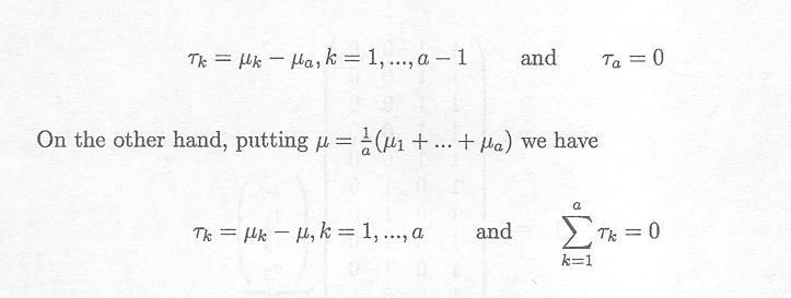
This model is advantageous if the primary interest is in differences in cell means, e.g., µk. µa, k = 1, ..., a . 1, or in differences between individual cell means and a reference or baseline value.
Note that since the model is overparameterised (in the sense that the model has a+1 parameters compared with a parameters in the cell means model) each choice of the reference value leads to some constraint (e.g. ta = 0 if µ = µa).
Therefore, µ can have different meanings depending on the implied restrictions. Its meaning can be made clear by defining µ in terms of the cell means.
Thus, putting µ, = µa we have
Example 2.2.1.1 The cell means model
We revisit Example 1.2.1. There are three different cell means, the mean PCV for animals that have been treated with a low dose (µl), a medium dose (µ2) and with a high dose (µ3) of the trypanocidal drug. There are 5 animals treated with the low dose (nl = 5), 4 with the medium dose (n2 = 4) and 5 animals with the high dose (n3 = 5).
This leads to the following model description in matrix form
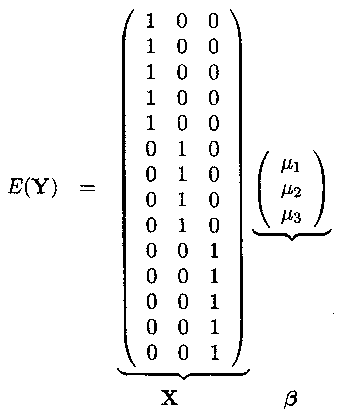
with YT = (Yll,Y12,Y13,Y14,Y15,Y21,Y22,Y23,Y24,Y31,Y32,Y33,Y34,Y35)
Example 2.2.1.2 The overparameterised model
We can rewrite the data structure of Example 1.2.1 as an overparameterised model
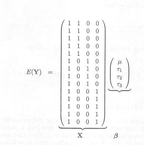
where t1 and t2 are interpreted as the differences between the low and the high dose (µl
. µ3) and the medium and the high dose (µ2
. µ3), respectively, if the constraint t3 = 0 is used, and
tk is equal to µk . µ (k = 1, 2, 3) if the constraint ![]() = 0 is used.
= 0 is used.
To obtain estimators for the terms of ß, the vector of cell means µ = (µ1, , µa)T in the cell means model, we try to solve the equation
Y=Xß
But in this form the set of N equations is insolvable since the number of parameters is a and the number of equations is N. We therefore obtain a solution based on the ordinary least squares criterion, i.e.,
obtain ß so that (Y . Xß)T (Y . Xß) is minimal
Minimising this expression with respect to means that we estimate the cell means so that the sum of squared differences between the observations and the cell means is minimal; in other words, estimators for the cell means are on average as close (in the least squares sense) to the observations as possible.
One can show that minimisation of least squares in this way is equivalent to solving the set of equations
XT Xß = XTY
This set of equations is called the set of normal equations. Now we have a equations and a parameters.
Example 2.2.1.3 Estimating parameters in the cell means model
For Example 1.2.1, we have
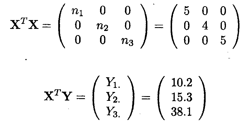
Note that rank (X)=3 (full rank), and that XTX is also of full rank. The inverse of XTX is
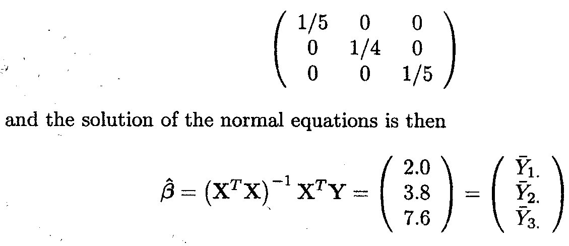
Thus, the cell means µk (k = 1, 2, 3) are
estimated by the means ![]() K of the observations Ykl (l = 1, ..., nk).
K of the observations Ykl (l = 1, ..., nk).
Parameter estimation in the overparameterised model is more complex. This is due to the fact that the (N x (a + 1)) design matrix X has rank a. Therefore, the design matrix is not of full rank. This is a direct consequence of the fact that the model is overparameterised. Therefore there is not a unique solution for the inverse of XTX and hence not a unique solution for the set of normal equations.
One solution is to impose a constraint on the parameters e.g. 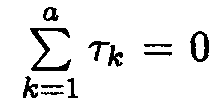 and reduce the matrix to full rank by reduce the matrix to full rank by substituting for
ta =. t1 . t2 - ... . Ta
. 1, say. This method is often applied in statistical programs. However, here we will consider the general case of using a generalised inverse of XTX.
This is a matrix G that satisfies
XTXGXTX = XTX
The general notation for the generalised inverse of a matrix A is A.. However, as a shorthand notation we use G to denote the generalised inverse of XTX. Such a generalised inverse is not unique. For each G we obtain a different solution of the set of normal equations. This solution takes the form
ß= GXT Y
There are different ways of obtaining a generalised inverse as is now shown by example.
Example 2.2.1.4 Estimating parameters in the overparameterised model
The matrix product XTX for the data set of Example 1.2.1 is given by

XTX is a (4 x 4) matrix and rank (XTX) = 3. Therefore the simple inverse of XTX does not exist and there is not a unique solution for the set of normal equations.
We discuss two ways to obtain a generalised inverse.
Method 1:
Assume that A is a square matrix of dimension (r x r) and that rank (A)=a (a < r). Partition A as
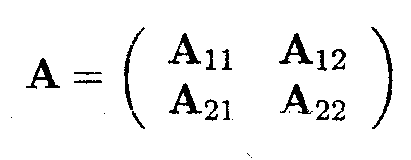
so that A11 is an (a x a) matrix of full rank.
Then one solution for A- in the equation AA-A = A is given by
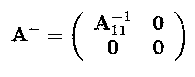
Note that each 0 in the expression for A- is a matrix.
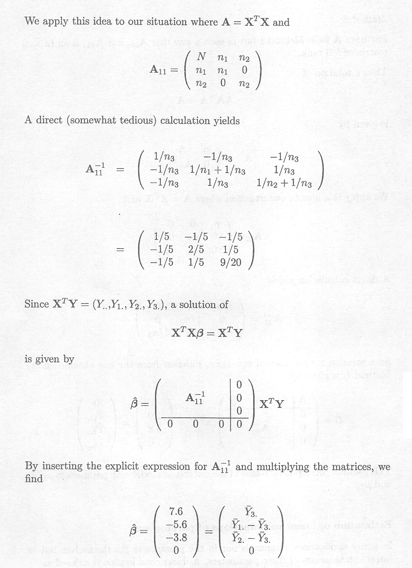
as one possible solution of the set of normal equations. This corresponds to the situation with µ = µ3 and t3 = 0.
Method 2:
Partition A as in Method 1 but in such a way that A22, not A11, is an (a x a) matrix of full rank.
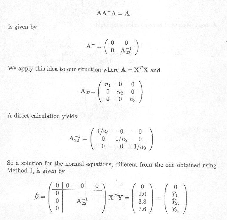
Then a solution of
 t
t
This solution corresponds to that of the cell means model with parameters µl, to µ2 and µ3.
Estimation of linear combinations of parameters
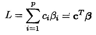
In many applications interest is not in the parameters, ßis themselves but in linear combinations of these parameters. A linear combination is defined as
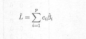
An estimate ![]() of a linear combination L can easily be obtained once parameter estimates are available as
of a linear combination L can easily be obtained once parameter estimates are available as
In the case of the cell means model estimation of any linear combination is straightforward.
Assume, for instance, in our example, that we want to estimate the difference between the low dose and the average of the medium and high doses. The vector product CTß is then given by

An estimate for this linear combination is given by

In the case of the overparameterised model, however, we have seen that different solutions for
ß can be obtained depending on the choice of the generalised inverse. In general we have that each solution gives a different value for ![]() . Linear combinations for which
. Linear combinations for which ![]() is invariant with respect to the choice of the generalised inverse are called estimable functions. Based on our example we further explain what we mean by estimable functions.
is invariant with respect to the choice of the generalised inverse are called estimable functions. Based on our example we further explain what we mean by estimable functions.
Example 2.2.1.5 Estimable functions
Consider the one-way overparameterised model
Y=Xß + e
with ßT = (µ,T1,T2,T3) and
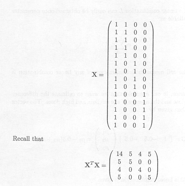
and that XT X is a (4 x 4)-matrix and rank (XT X)=3. With G a generalised inverse of XT X we have that
![]() G=GXT
Y
G=GXT
Y
is a solution of the set of normal equations
XTXß = XTY
It is easy to show, for example, that G1 and G2 are generalised inverses for XTX, where
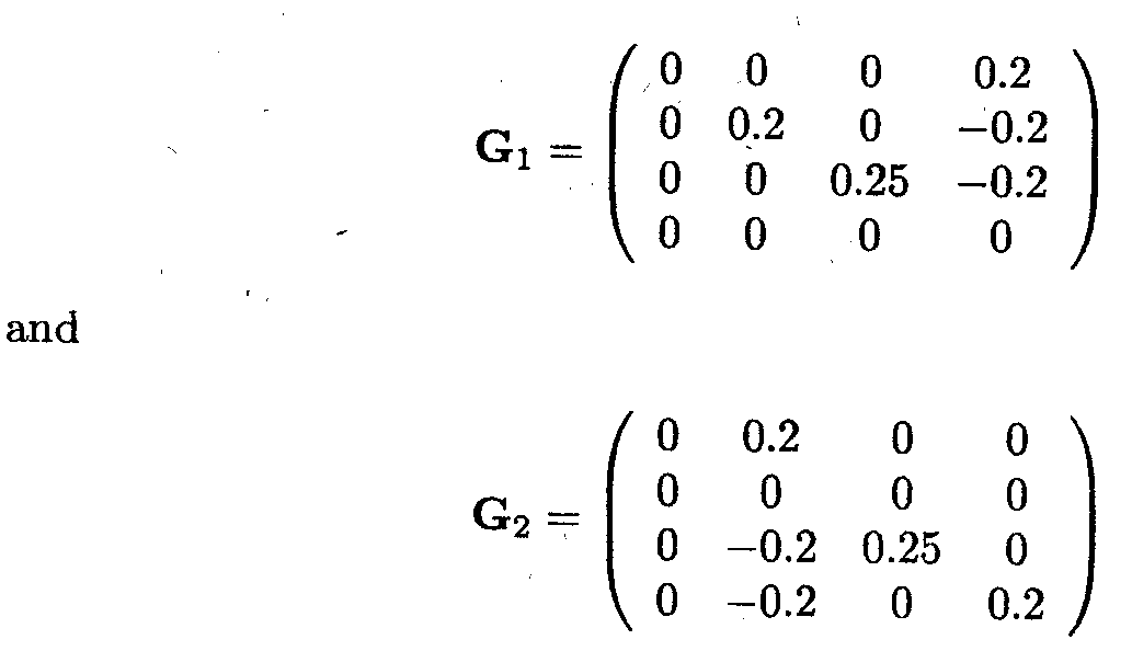
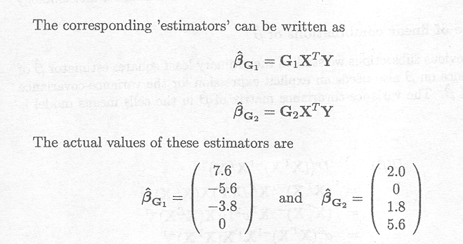
From this example it is clear that 'estimators' for µ, tl, t2 and t3 depend on what has been chosen as the generalised inverse. The following table gives for five choices of G (not given explicitly) the actual values for the estimators of the parameters and of certain linear functions of the parameters.
Table 2.2.1.1 Solutions for parameters and linear combinations of parameters based on different generalised inverses
Solution | |||||
Parameter |
1 |
2 |
3 |
4 |
5 |
| µ | 0 |
4.46 |
2.0 |
7.6 |
150 |
ti |
2.0 |
-2.46 |
0 |
-5.6 |
-148.0 |
t2 |
3.8 |
-0.66 |
1.8 |
-3.8 |
-146.2 |
t3 |
7.6 |
3.14 |
5.6 |
0 |
-142.4 |
Linear combination | |||||
t1 + t2 |
5.8 |
-3.12 |
1.8 |
- 9.4 |
- 294.2 |
(t1 + t2 + t3) /3 |
4.46 |
0.02 |
2.46 |
- 3.13 |
- 145.53 |
t1 . t2 |
-1.8 |
-1.8 |
-1.8 |
- 1.8 |
- 1.8 |
µ + t1 |
2.0 |
2.0 |
2.0 |
2.0 |
2.0 |
µ + t3 |
7.6 |
7.6 |
7.6 |
7.6 |
7.6 |
We see that the actual values of the estimators of the parameters change with the choice of G, as we have already discussed before, but we also see that the value for some linear combinations of µ, tl, t2, t3 is the same whatever G is chosen. Such linear combinations are called estimable functions. It turns out that linear combinations of parameters that are relevant in practice (e.g. t1 . t2, µ + t1, µ + t2) are estimable. Furthermore, estimable functions can always be written as a function of the cell means. For instance, if the restriction equals t3 = 0, then it follows that µk = µ + tk, and thus, as an example, t1 - t2 = µ1 - µ2. On the other hand, no such relationship exists for tl + t2.
Variance of linear combinations of ![]()
In the previous subsections we studied the ordinary least squares estimator
![]() of
of ![]() Inference on
Inference on ![]() also needs an explicit expression for the variance-covariance matrix of
ß. The variance-covariance matrix of
also needs an explicit expression for the variance-covariance matrix of
ß. The variance-covariance matrix of ![]() in the cells means model is given by
in the cells means model is given by
D(![]() ) = D ((XTX)-1XTY)
) = D ((XTX)-1XTY)
= (XTX)-1XTD(Y)X(XTX)-1
= (XTX)-1XTs2INX(XTX)-1
= s2(XTX)-1XTX(XTX)-1
s2(XTX)-1
whereas in the overparameterised model it is given by
D(![]() ) = D (GXTY)
) = D (GXTY)
= GXTD(Y)XGT
= s2GXTXGT
Note that the latter expression is not invariant for G. This means that the variance-covariance matrix of
![]() depends on the particular choice of the generalised inverse. In the previous section we defined estimable parameters as those linear combinations of ß (i.e. L = cTß,) for which the corresponding estimator
depends on the particular choice of the generalised inverse. In the previous section we defined estimable parameters as those linear combinations of ß (i.e. L = cTß,) for which the corresponding estimator ![]() = CT
= CT
![]() is invariant with respect to the choice of G.
is invariant with respect to the choice of G.
One can show that cTß is estimable if and only if cTß
= tTX where t is a N x 1 vector with each element equal to some real number. Based on this fact it can be shown (as described in Appendix E) that the variance of ![]() = cT
= cT![]() is invariant to the choice of G and given by
is invariant to the choice of G and given by
Var(cT![]() ,) = s2tTXGXTt
,) = s2tTXGXTt
For the cell means model we simply obtain
Var(cT![]() ) = s2cT (XTX)-1 c
) = s2cT (XTX)-1 c
The variance-covariance expression requires estimation of s2. The least squares estimator is based on the sum of squared differences between the observations and estimated cell means µk = k. given by

It can easily be shown that this is an unbiased estimator of s2, whereas the log-likelihood estimator given by

is a biased estimator of s2. We will come back to this issue in more detail in Section 2.4.
The value of s2 can then be used in the estimation of
var (cT![]() ) and the
(1- a )100% confidence interval for cTß is given by
) and the
(1- a )100% confidence interval for cTß is given by

Note that the t-distribution with N . a degrees of freedom is used here, and not the standard normal distribution, because an estimate s2 of s2 was used to calculate the variance of the estimated parameter, which introduces additional uncertainty, taken care of by the t-distribution.
Example 2.2.1.6 Confidence intervals
If the cell means model for the data set of Example 1.2.1 is used, the variance-covariance matrix of ![]() is given by
is given by

Therefore, the variance of the estimate ![]() , for instance, is given by
, for instance, is given by

An unbiased estimator for s2 is given by

and an estimate of the variance of the estimate ![]() is
is

A 95% confidence interval for µ1 is then given by

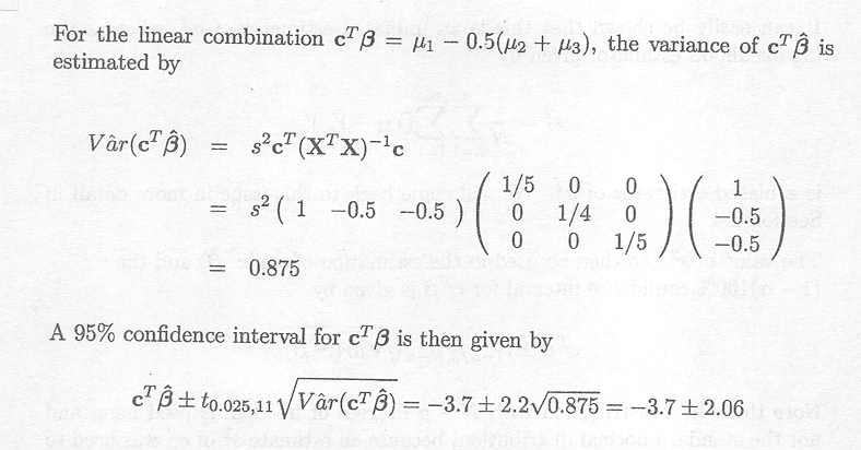
We can also use the overparameterised model to find the same estimates and confidence intervals.
Now the vector of fixed effects is given by
ßT = (µ t1 t2 t3 )
and suppose the linear combination of interest is given by
cTß = (1 1 0 0 )ß
Assume that the Gl generalised inverse is used to find a solution for ß
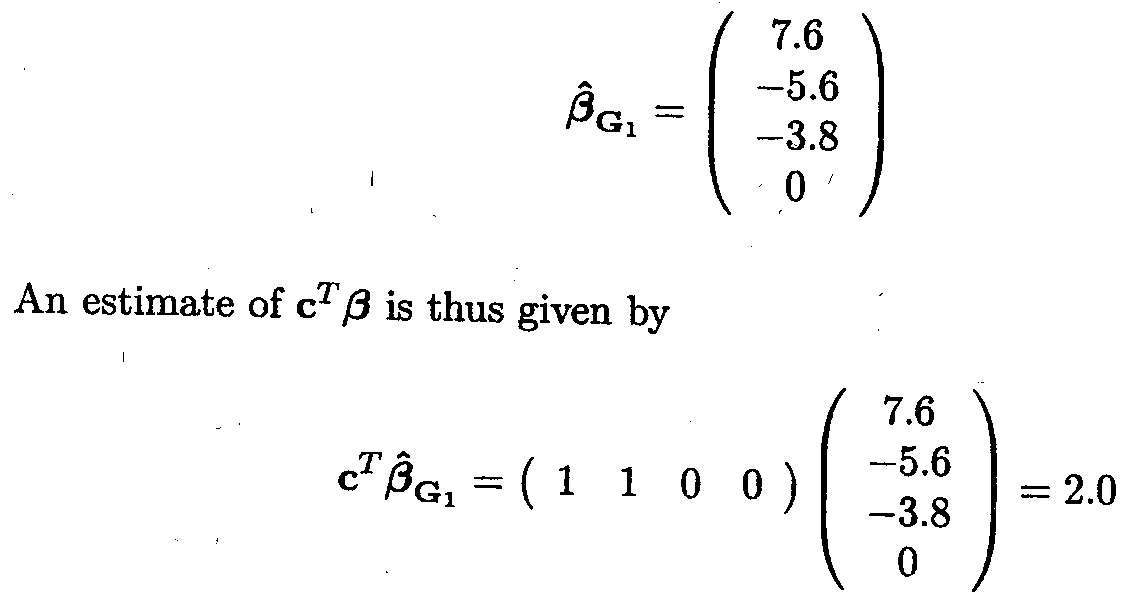
The variance-covariance matrix of ![]() G1 can be estimated by
G1 can be estimated by
![]() (
(![]() G1) = s2G1XTXG
G1) = s2G1XTXG![]()
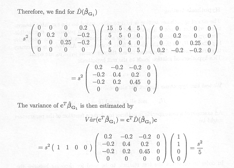
Both cT![]() Gl and the estimated variance
Gl and the estimated variance ![]() (cT
(cT![]() G1) are thus the same as for the cell means model. This is due to the fact that cTß
is an estimable function and both its estimate and its estimated variance are independent of the particular choice of the generalised inverse.
G1) are thus the same as for the cell means model. This is due to the fact that cTß
is an estimable function and both its estimate and its estimated variance are independent of the particular choice of the generalised inverse.
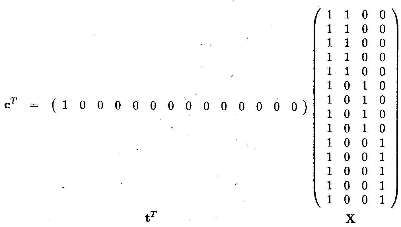
To show that cTß is estimable, we need to show that cTß can be written as tTX:
The aim of hypotheses testing is to determine, based on the available observations, whether or not a hypothesised relation between parameters is plausible. The hypothesised relation is called the null hypothesis (H0). The alternative hypothesis (Ha) is that the claim is false. For one-way ANOVA it is customary to start by determining whether or not the cell means µl,.., µa are equal. This hypothesised relation leads to the null hypothesis
H0 :µ1 = ... = µa
We test this hypothesis against the alternative
Ha : not all µk equal (k = 1, ..., a)
An example of a more specific hypothesis involving a function of the parameters might be
H0 : µ1 = (µ2 + µ3) /2
Ha : µ1 ? (µ2 + µ3) /2
In order to construct the test statistic to be used for choosing between the alternatives H0 : µl = ... = µa and Ha : not all µk equal, the total sum of squares of all the observations
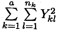 in the data set is decomposed into different terms in the following table.
Table 2.2.1.2 Decomposition of total sum of squares
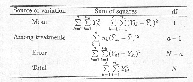
The total number of degrees of freedom is equal to the total number of observations, and can be subdivided in a similar way as the sum of squares. The among treatments sum of squares (SSTR) has
a . 1 degrees of freedom as there are a estimated deviations![]() k. –
k. – ![]() but one
degree of freedom is lost because the deviations are not independent since
but one
degree of freedom is lost because the deviations are not independent since ![]()
The error sum of squares (SSE) has N – a degrees of freedom as for each treatment there are nk
– 1 independent deviations in the sum
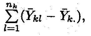 and, having
a such levels, this gives

The mean squares can be obtained by dividing their respective sums of squares by their associated degrees of freedom:
MSTR = SSTR/(a . 1) and MSE = SSE/(N . a)
The first important point to note is that the expected values of MSTR and MSE are both equal to s2 under the null hypothesis, whereas the expected value of MSTR is greater under the alternative hypothesis.
Indeed the expected values can be shown to be as follows (see Appendix G)
E(MSE) = s2
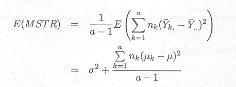
Thus, a test can be based on the comparison between these two mean squares.
Another important point to note is that SSTR and SSE divided by s2 both follow a Chi-squared distribution under the null hypothesis.
Thus, under the null hypothesis

Owing to the fact that SSE/s2 and SSTR/s2 are Chi-squared distributed and independent from each other, the ratio
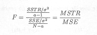
has a F-distribution with a . 1 and N . a degrees of freedom.
Thus,
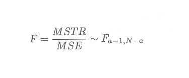
We can therefore use the F-statistic to test the general hypothesis.
More specific hypotheses can be tested in the same way if an appropriate sum of squares can be found for which the expected value is equal to E(MSE) under the null hypothesis, and is greater than E(MSE) under the alternative hypothesis.
In this way all possible linear combinations of parameters can be tested.
Example 2.2.1.7 Testing hypotheses
The total sum of squares and the degrees of freedom of the observations of the data set shown in Example 1.2.1 can be divided as shown in the following table.
Table 2.2.1.3 Decomposition of total sum of squares for Example 1.2.1
Source of variation |
Sum of squares |
df |
Mean square |
Mean |
289.25 |
1 |
289.25 |
Among doses |
80.73 |
2 |
40.36 |
Error |
30.91 |
11 |
2.81 |
Total |
400.86 |
14 |
The value of the F-statistic is
F = ![]() =
14.36
=
14.36
and can be used to test the general hypothesis that the three doses give the same mean response in PCV.
Under this null hypothesis the F-statistic is distributed as
F ~ F2,11
Therefore, the P-value is given by
Prob (F2,11 14.36) = 0.0009
So even at the 0.1% significance level the null hypothesis can be rejected.
Now consider the more specific hypothesis testing problem
H0 : µ1 = 0.5(µ2 + µ3)
Ha : µ1 0.5(µ2 + µ3)
The distributional assumptions of the estimate of µ1 - 0.5(µ2 + µ3) can be used to derive the appropriate F-statistic. An estimate for µ1 - 0.5(µ2 + µ3) is given by ![]() l.-0.5(
l.-0.5(![]() 2.+
2.+![]() 3.).
3.).
Under the null hypothesis, it has been shown that

As the F-distribution can be obtained by squaring the t-distribution, the following distributional property holds
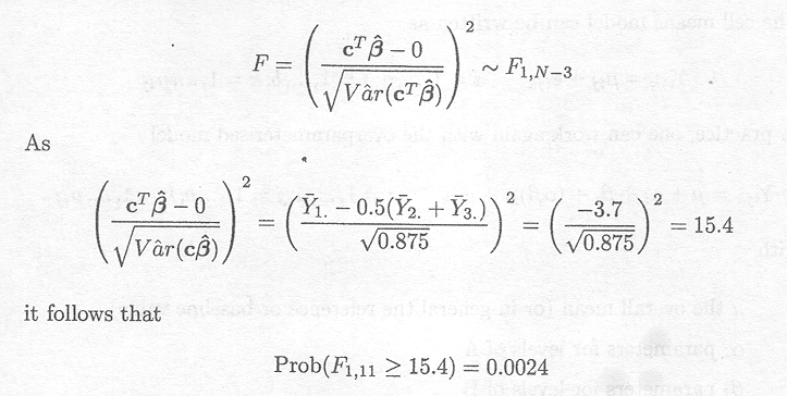
Thus the null hypothesis is rejected (P< 0.01).
The decomposition of the sum of squares and degrees of freedom and application of the statistical tests can easily be obtained from the GLM procedure in SAS. The program that generates the output discussed above is shown in Appendix B.2.1.
The following table is extracted from the generated output
Dependent Variable: PCV
Source |
df |
Sum of Squares |
Mean Square |
F value |
Pr > F |
Model |
2 |
80.73 |
40.38 |
14.37 |
0.0009 |
Error |
11 |
30.91 |
2.81 |
||
Corrected Total |
13 |
111.63 |
|||
Source | |||||
DOSE |
2 |
80.73 |
40.36 |
15.17 |
0.0009 |
Contrast | |||||
1 vs mh |
1 |
43.39 |
43.39 |
15.44 |
0.0024 |
Parameter |
Estimate |
T for H0: Parameter=0 |
Pr > /t/ |
Standard error of estimate | |
1 vs mh |
. 3.68 |
. 3.93 |
0.0024 |
0.937 | |
The corrected total sum of squares is the total sum of squares minus the sum of squares for the mean described earlier, and represents the sum of squares of deviations of observations about the overall mean

The description of one-way ANOVA models extends easily to two-way and multiway ANOVA.
Instead of one independent variable, the model now contains two independent variables, A and B, each having a number of levels a and b respectively.
The cell means model can be written as
Yijk = µij + eijk i= 1, .. , a; j = 1, .. , b; k = 1, .. , nij
In practice, one can work again with the overparameterised model
Yijk = µ + ai +ßj +(aß)ij + eijk i = 1,, a;j = 1,, b;k = 1, , nij
with
µ the overall mean (or in general the reference or baseline value)
ai parameters for levels of A
ßj parameters for levels of B
(aß)ij parameters describing interactions between levels of A and B
eijk independent homoscedastic normal errors (with zero mean).
Example 2.2.2.1 Two-way ANOVA model specification
Assuming that there are two observations for each treatment combination (nij = 2 for each i and j) and that each of the two independent variables has two levels, the cell means model in matrix notation is given by
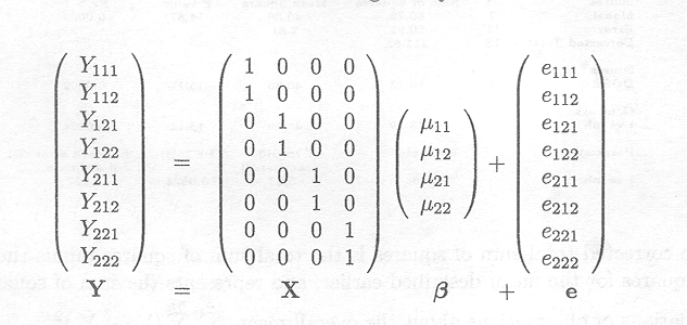
X is the design matrix, rank(X)= 4. The dimension of X is (N x 4), with N=8 the total number of observations.
The design matrix X in the overparameterised model becomes
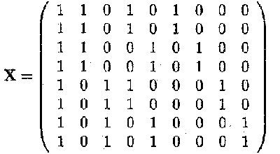
and ßT = (µ a 1 a 2 b 1 b 2 (ab )11 (ab )12 (ab )21 (ab )22)
The vectors Y and a are the same as before.
Note that the dimension of X is (8 x 9) but rank(X)= 4. So X is not a full rank matrix.
Mixed models and fixed effects models study the relationship between a response and one or more independent variables or factors. For a fixed effects factor we assume there to be only a finite set of levels that can be represented and that inferences are to be made only concerning the levels defined for the study. For a random effects factor, however, we assume that there is an 'infinite' set of levels (a population of levels) and we think about the levels present in the study as being a sample from that population. In Section 2.3.1 it is explained how a data set can be described in the mixed model framework by using a notation for each separate observation. All the examples introduced in Chapter 1 are revisited in Section 2.3.2 and statistical models axe defined in the mixed model notation. In Section 2.3.3 a general matrix form for the mixed model is introduced and the matrix form of some of the examples is discussed in detail.
We introduced in Section 2.2.1 the following overparameterised fixed effects model
Ykl = µ + tk + ekl, k = 1, ..., a; l = 1, ..., nk
where µ and the tk s are unknown parameters.
Assume now that we have again only one factor, but this time it is a random effects factor. The model description is similar
Ykl = µ + tk + ekl, k = 1,...,a;l = 1, ...,nk
but t1,..., ta are considered to be a random sample from a normally distributed population with mean zero and variance
s![]() , i.e. tk ~ N(0, s
, i.e. tk ~ N(0, s![]() ) and tl , ..., ta are independent. Furthermore it is assumed that every ekl is independent from every tk.
) and tl , ..., ta are independent. Furthermore it is assumed that every ekl is independent from every tk.
This model is called a random effects model; it only contains an overall mean parameter µ as a fixed effect. Thus a model with only one factor in addition to the mean can be either a fixed effects model or a random effects model.
When there are two or more factors, one may be a random effects and the other a fixed effects factor; the model is then called a mixed model. We now revisit the examples discussed in Chapter 1 and for each of them give a model description.
Comparing three doses of a drug: a completely randomised design
The data structure of Example 1.2.1 can be described by the following statistical model
Ykl = µ + tk + ekl
where, for k = 1, 2, 3; l = 1, ..., nk,
Ykl is the difference in PCV (=PCVafter - PCVbefore)
µ is the overall mean
tk is the effect of the low (t1), medium (t2) or high (t3) dose of Berenil
ekl is the random error of animal l given dose k
Both µ and tk are fixed effects. For the random effects ekl we assume independence and
ekl ~ N(0, s2)
In words: the random error ekl describes the deviation of the observation Ykl from the expected value µk = µ + tk; these errors are assumed to be independent and normally distributed with mean 0 and variance s2. The model is a fixed effects model.
Comparing two doses of a drug: a randomised block designThe data structure of Example 1.2.2 can be described by the following statistical model
Yikl = µ + hi + tk + eikl
where, for i =1, 2, 3; k =1, 2; l =1, ..., nik,
Yikl is the difference in PCV (=PCVafter - PCVbefore)
µ is the overall mean
hi is the effect of herd i
tk is the effect of the high (t1) or low (t2) dose of Berenil
eikl is the random error of animal l given dose k in herd i
Both µ and tk are fixed effects. For hi, however, we have a choice; we can either assume it to be a fixed effect so that inference can apply only to the herds in question; alternatively, we can assume that the herds have been selected from a population of herds. In this example we shall assume the latter. Thus, both hi and eikl are random effects.
The assumptions are
the hi are iid N(0,s![]() )
)
the eikl are iid N(0,s2)
the hi and eikl are independent
Thus, the random effect hi describes the effect of a particular herd on
the response variable. The effect of a particular herd is assumed to belong to a
normal distribution with mean zero and variance s![]() . In this example interest is
thus not in the particular herds, but rather that conclusions should be valid
for the whole population.
. In this example interest is
thus not in the particular herds, but rather that conclusions should be valid
for the whole population.
Comparing two drugs: a completely randomised design with repeated observations
The data structure of Example 1.2.3 can be described by the following statistical model
Yijl = µ + di + hij + eijl
where, for i = 1, 2; j = 1, 2; 1 = 1, ..., nij,
Yijl is the difference in PCV (=PCVafter - PCVbefore)
µ is the overall mean
di is the effect of the Berenil (d1) or Samorin (d2)
hij is the effect of herd j which receives drug i
eijl is the random error of animal l in herd j to which drug i has been assigned.
Both µ and di, are fixed effects, whereas hij and eijl are random effects; the assumptions are
the hij are iid N(0,s![]() )
)
the eijkll are iid N(0,s2)
the hij and eijkl are independent
Thus the random effect hij describes the effect of a particular herd on
the response variable, and the selection of particular herds is assumed to be a
random sample from a normal distribution with variance s![]() . Although the model is similar
to the model of the previous example, there is a substantial difference. In this
case the treatment is assigned to animals in a herd as a whole. For this reason
we use the notation hij,
which means that the herd factor is 'nested' in the drug factor, so that
each animal in a herd nested in drug i receives drug i.
. Although the model is similar
to the model of the previous example, there is a substantial difference. In this
case the treatment is assigned to animals in a herd as a whole. For this reason
we use the notation hij,
which means that the herd factor is 'nested' in the drug factor, so that
each animal in a herd nested in drug i receives drug i.
Comparing two drugs at two different doses: two sizes of experimental units
The data structure of Example 1.2.4 can be described by the following statistical model
Yikl = µ + di + hij +tk +(dt)ik+eijkl
where, for i = 1, 2; j = 1, 2; l = 1, ..., nij,
Yijkl is the difference in PCV (=PCVafter - PCVbefore)
µ is the overall mean
di is the effect of the Berenil (d1) or Samorin (d2)
hij is the effect of herd j which receives drug i
tk is the effect of the high t1 or low t2 dose
(dt)ik is the interaction effect between drug and dose
eijkl is the random error of animal l at dose k in herd j to which drug i has been assigned
Both µ,di Tk,(dT)ik are fixed effects, whereas hij and eijl are random effects.
The assumptions are
the hij are iid N (0,
s![]() )
)
the eijkl are iid N (0, s2)
the hij and eijl are independent
Thus, the random effect hij describes again the effect of a particular herd on the response variable.
Comparing two drugs at two different doses: a split plot design
The data structure of Example 1.2.5 can be described by the following statistical model
Yijk = µ + di + rj + hij + Tk + (dT)ik + eijk
where, for i = 1, 2; j = 1, ..., 6; k = 1, 2,
Yijk is the difference in PCV (=PCVafter - PCVbefore)
µ is the overall mean
di is the effect of the Berenil (d1) or Samorin (d2)
rj is the random effect of region j
hij is the random effect of the herd within region j to which level i of the drug has been assigned
Tk is the effect of the high (Ti) or low (T2) dose
(dT)ik is the interaction effect between drug and dose
eijk is the random error of the average response of animals from region j to which the ik drug-dose treatment has been applied
Both µ., di, Tk and (dT)ik are fixed effects, whereas rj, hij and eijk are random effects; the assumptions are
the rj are iid N(0,
s![]() )
)
the hij are iid N(0, s![]() )
)
the eijk are iid N(0,s2)
the rj , hij and eijk are independent
Thus the random effect rj describes the effect of a particular region on the response variable. The random effect hij describes the effect of herd within a region on the response variable.
Variation in ELISA data
The data structure of Example 1.2.6 can be described by the following statistical model
Yijk = µ + ai + tj + eijk
where, for i =1, ..., 4; j = 1, ...,11; k = 1, 2,
Yijk is the OD value
µ is the overall mean
ai is the effect of animal i
tj is the effect of time j
eijk is the random error of measurement k at time j on animal i
In this case ai is assumed to be a random effect; provided there is no systematic pattern of changes in OD with time, we can also assume that tj is a random effect. Thus, for the random effects ai, tj and eijk we assume
the ai are iid N(0, s![]() )
)
the ti
are iid N(0, s![]() )
)
the eijk are iid N(0,s 2)
the ai, ti and eijk are independent
Since the overall mean is the only fixed effect, this is a random effects model. The interest of the investigator is in the magnitudes of the different sources of variability on the OD value.
Helminth-resistance in sheep
The data structure of Example 1.2.7 can be described by the following statistical model
Yij = µ + si + eij
where, for i = 1, ..., 8; j = 1, ..., nii,
Yij is the weaning weight
µ is the overall mean
si is the effect of the sire i
eij is the random error of lamb j of sire i
In this case, there is only one fixed effect, the overall mean µ. The other effects si and eij are random effects.
The assumptions are
the si are iid N(0,
s![]() )
)
the eij are iid N(0,s2)
the si and eij are independent
The model is a random effects model. For this example, interest is in the sources of variability as well as in actual responses of the specific sires. It will be shown later how these two goals can be met together.
Breed differences in susceptibility to trypanosomosis
The data structure of Example 1.2.8 can be described by the following statistical model
Yikl = µ + ,ßi0 +ßil t + aik + eikl
where, for i = 1, 2; k = 1, ..., 6; l = 1, ...14,
Yikl is the PCV
µ is the overall mean
ßio is the intercept of the regression line for breed i
ßil is the slope of the regression line for breed i
aik is the effect of animal k belonging to breed i
eikl is the random error of measurement l on animal k belonging to the breed i
There are thus five fixed effects, the overall mean and the intercepts and the slopes for the two breeds. Both aik and eikl are random effects. The assumptions for the random effects are
the aik are iid N(0,s![]() )
)
the eikl are iid N(0,s2)
the aik and eikl are independent
The mixed model examples, given in Section 2.3.2, can also be written in matrix notation. The matrix form of a mixed model collects the fixed effects in a vector , and the random effects in a vector u, and finally the random error term, which is also a random effects factor, in the vector e. A formal definition is
Y = Xß+Zu + e
with X the known design matrix for the fixed effects and Z the known design matrix for the random effects.
The matrix representation for Example 1.2.2 is as follows
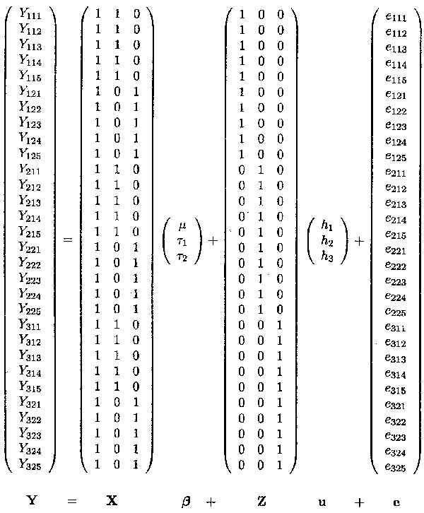
The example contains the mean, the dose factor which is a fixed effects factor at two levels, the herd factor which is a random effects factor at 3 levels and finally the random error term. The overall mean µ and the two fixed dose effects, tl and t2, are contained in the ß vector, whereas the three random herd effects hl, h2 and h3 are contained in the u vector.
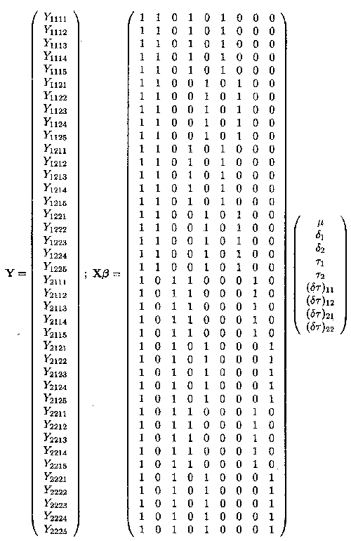
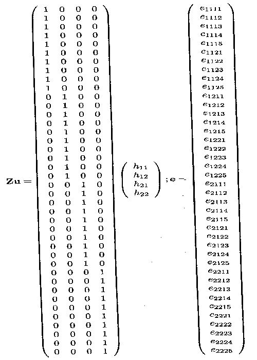
Example 1.2.4 contains the dose factor and the drug factor which are both fixed effects factor at two levels, the herd factor which is a random effects factor at 4 levels and finally the random error term. The overall mean µ., the two fixed dose effects, Tl and T2, the two fixed drug effects, d1 and d2 and the interaction effects (dT)11, (dT)12, (dT)21 and (dT)22 are contained in the ß vector, whereas the four random herd effects h11, h12, h21 and h22 are contained in the u vector.
This data structure can again be put in matrix form Y = Xß + Zu + e. The different parts are shown on the two next pages.
The X matrix can be divided in four parts, the first part is the vector Xµ, consisting of ls. The second part is the Xd matrix containing the two vectors corresponding to d1 and d2. The third part is the XT matrix containing the two vectors corresponding to Tl and T2. The last part is the Xy matrix containing the four vectors corresponding to (dT)11, (dT)12, (dT)21 and (dT)22.
It has been demonstrated how different variance components describe at different levels the variability in observations with a mixed model structure. The variance-covariance matrix of Y where
Y = Xß + Zu + e
is obtained as follows.
The first part of the model, Xß , does not contribute to the variance of Y as it only contains fixed effects. Furthermore, the
assumptions are made that each element u1 in the
vector u is a random effect which comes from a
normal distribution with mean 0 and variance s![]() , and that the elements are
independent from each other and that the covariances among the elements of u are thus zero. The variance-covariance matrix for u is therefore given by a diagonal matrix D(u). All the elements in the
vector u are assumed to be independent from the
elements in e. We
further have that the elements in e are also
normally distributed with mean 0 and variance s2 and are independent
from each other. Given these assumptions, the variance-covariance matrix of Y is then given by
, and that the elements are
independent from each other and that the covariances among the elements of u are thus zero. The variance-covariance matrix for u is therefore given by a diagonal matrix D(u). All the elements in the
vector u are assumed to be independent from the
elements in e. We
further have that the elements in e are also
normally distributed with mean 0 and variance s2 and are independent
from each other. Given these assumptions, the variance-covariance matrix of Y is then given by
D(Y) = D(Zu) + D(e) = ZD(u)ZT + s2 IN
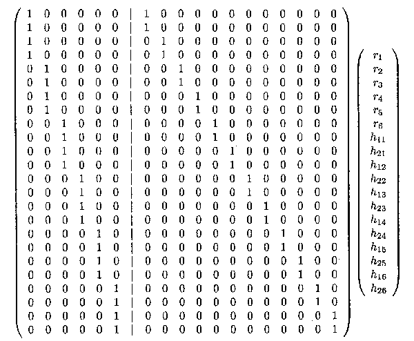
We revisit Example 1.2.5. The vector u consists of 18 random effects, 6 random effects for the regions (rl .... r6), 12 random effects for the herds (h11, h21, h12, h22, ..., h16, h26) whereas the Z matrix is a (24 x 18) matrix.
Note that the matrix product can also be written as the sum of two different matrix products. The first 6 entries of the u vector and the first 6 columns of the Z matrix can be defined as ur and Zr respectively and the remaining entries of a and Z as uh and Zh, respectively. Thus, ur and Zr contain all the information with regard to the regions, whereas uh and Zh contain all the information with regard to the herds within regions. Thus

For the vector of observations sorted by region, given by
YT = (Y111 , Y112 , Y211, Y 212, ..., Y161, Y162, Y261, Y262), the matrix product Zu is shown below.
As it is assumed that ur and uh are independent from each other, the variant of Zu can be obtained as
D(Zu) = D(Zrur) + D(Zhuh) = ZrD(ur)Z![]() + ZhD(uh)Z
+ ZhD(uh)Z![]()
Given that the different entries in ur are independent from each other, the variance-covariance matrix of ur. is given by
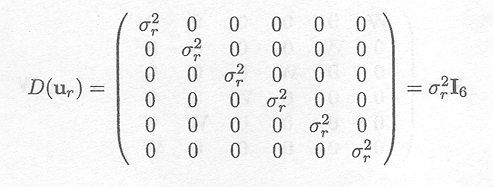
In a similar way, the variance-covariance matrix of uh can be obtained as
D(uh) = s![]() I12
I12
Therefore, the variance-covariance matrix of Y is given by
![]()
Both Zr and Zh can be written in a simpler form as (Appendix C)
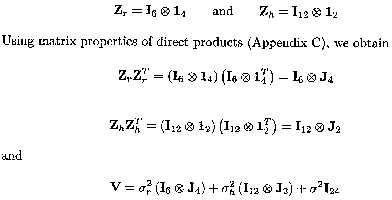
Define Yj as the vector
containing the four observations from region j, Y![]() =
(Yljl,Ylj2,Y2j1,Y2j2)
=
(Yljl,Ylj2,Y2j1,Y2j2)
For D(Yj) = W, the variance-covariance matrix of Yj, we have

Thus, the variance of an observation corresponds to
s2+s![]() +s
+s![]() , the covariance between two
observations from the same herd equals s
, the covariance between two
observations from the same herd equals s![]() +s
+s![]() and finally, the covariance
between two observations from the same region, but from different herds,
corresponds to s
and finally, the covariance
between two observations from the same region, but from different herds,
corresponds to s![]() .
.
The full variance-covariance matrix is then equal to
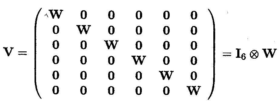
Thus, the different variance components prevail in the variance-covariance matrix of the vector Y. Actually, the only variable elements in the matrix V are the different variance components. In order to derive an estimate of the matrix V, estimates of the variance components axe needed for insertion into V. In the next subsection it is discussed how estimates of variance components can be obtained.
There exist different methods to estimate variance components. Only likelihood based estimators are considered here (Harville, 1977). An excellent monograph on likelihood is written by Edwards (1972). Estimation methods for variance components based on other criteria are well described by Searle et al. (1992).
We assume the following distributional assumptions for the observation vector Y
Y ~ MVN(Xß, V)
The likelihood of Y is then given by

where ? V? means the determinant of the matrix V (see Appendix C).
The only unknowns in V are
the variance components s![]() ,
..., s
,
..., s![]() , with d the number of variance components.
, with d the number of variance components.
Thus the log-likelihood can be rewritten as
lY (, V) = lY (, s![]() ,
..., s
,
..., s![]() )
)
Maximum likelihood estimators can then be obtained by
maximising this expression with regard to ß and
s![]() , , s
, , s![]() Differentiating the
log-likelihood with respect to the different parameters and setting the result
equal to 0 leads to the maximum likelihood estimator for each parameter.
Differentiating the
log-likelihood with respect to the different parameters and setting the result
equal to 0 leads to the maximum likelihood estimator for each parameter.
Differentiating the log-likelihood with respect to ß gives
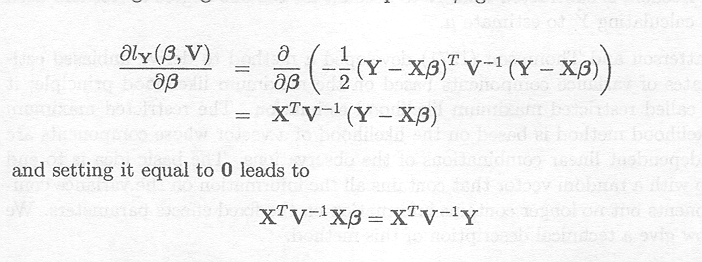
Thus a solution for ß can be obtained as a function of the unknown variance components. This solution can then be inserted into the remaining differential equations in order to lead to a solution for the variance components. In some cases, however, the value that maximises the log-likelihood turns out to be negative (Searle et al., 1992). Although sometimes a negative variance component makes sense (Henderson, 1953; Nelder, 1954), e.g., if the variance component corresponds to a correlation (see Example 3.3), in most cases the parameter space for the variance components is restricted to the interval containing only positive numbers and zero. If a variance component becomes negative, it is usually set to zero and it can be shown (Searle et al., 1992) that, within the restricted region, the zero estimate corresponds to the maximum likelihood estimate. SAS does this by default (SAS Institute Inc. Cary, NC, 1996; Littell et al., 1996). In what follows, the term maximum likelihood estimators is used for the maximum likelihood estimators in the restricted parameter space.
The maximum likelihood estimators of the variance components are biased. The estimate will on average be smaller than the population value. The reason for this is that in the estimation procedure the existence of fixed effects is ignored, and the degrees of freedom used in deriving the estimators do not adjust for this.
The most straightforward example is the estimator of the variance of a sample YT = (Y1,...,YN) of a univariate normal distribution N(µ,s 2). The unbiased estimator of s2 is given by

If, however, the maximum likelihood criterion is used, the estimator of s2 is given by
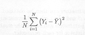
Thus, this estimator underestimates s2. For the unbiased estimator, one degree of freedom is subtracted from N to account for the one degree of freedom used in calculating Y to estimate µ.
Patterson and Thompson (1971) developed a method to derive unbiased estimates of variance components based on the maximum likelihood principle; it is called restricted maximum likelihood estimation. The restricted maximum likelihood method is based on the likelihood of a vector whose components are independent linear combinations of the observations. The basic idea is to end up with a random vector that contains all the information on the variance components but no longer contains information on the fixed effects parameters. We now give a technical description of this method.
Since X is the design matrix for the overparameterised model, it is not of full rank. The rank of X is the number of cell means in the model (the total degrees of freedom associated with the fixed effects). We call this rank r, i.e., rank(X)=r.
A set of linear combinations, denoted as KY, is derived, where K is a (N. r, N) matrix of full rank (see Appendix C)
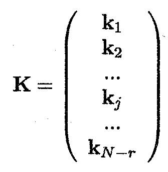
and which obeys the following equation
E(KY) = 0
As E(KY) = KXß, it follows that for each individual linear combination
kj X = 0
The individual linear combinations kjY axe called error contrasts (Harville, 1974; Harville, 1977).
As Y is assumed to be normally distributed MYN(X,V), it follows that
KY ~ MVN(0, KVKT)
The restricted maximum likelihood criterion is based on the likelihood of KY. This likelihood does not contain fixed effects and furthermore contains fewer terms (N . r) as compared to the likelihood of the observation vector Y. Maximising the likelihood of KY will yield the restricted maximum likelihood estimators for the variance components.
Assume that a sample is taken from a large herd to obtain an estimate of the average body weight of animals in that herd. Apart from the estimate of mean body weight also its variability is of interest. The weight of an animal can be assumed to be normally distributed N(µ,s2). Denote the sample as Y = (Y1, ..., YN)T; the observations are assumed to be independent. Therefore the variance covariance matrix of Y is
V =s2IN
and
Y = MVN(µ1N, s2IN)
The log-likelihood of Y is given by

Differentiating this expression first with respect to µ, we obtain

and setting it equal to 0 gives
(Y . µ1N)1N = 0
leading to

Differentiating the log-likelihood of Y with regard to s2, we obtain
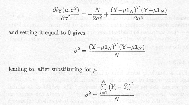
When using the restricted maximum likelihood criterion, a matrix K must be found that satisfies the aforementioned specifics. One such K (of dimension (N . 1, N)) is given by
K = (IN . 1 . N. 1JN. 1 .N . 11N . 1)

It can easily be shown that the (N - 1) rows are linearly independent, and that each row satisfies kj X = 0 and therefore
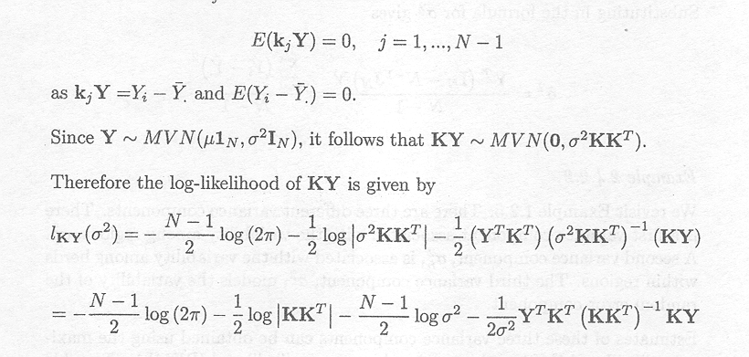
Differentiating this log-likelihood expression with regard to s2 and setting it equal to 0 gives

It can be shown (Searle et al., 1992) that, in general,
KT (KKT). 1 K = IN . X(XTX). 1XT
for any appropriate choice of K.
In our example for body weight, the X matrix consists simply of a vector of 1's of length N, 1N.
Thus
XT X = N and (XTX). 1 = 1/N
and furthermore
XXT = JN
Therefore
KT (KKT) . 1
K = IN .![]()
Substituting in the formula, for s2 gives

We revisit Example 1.2.5. There are three different
variance components. There is a first variance component associated with the
variability among regions, s![]() . A
second variance component, s
. A
second variance component, s![]() ,
is associated with the variability among herds within regions. The third
variance component,s 2,
models the variability of the random error component.
,
is associated with the variability among herds within regions. The third
variance component,s 2,
models the variability of the random error component.
Estimates of these three variance components can be obtained using the maximum likelihood (ML) or the restricted maximum likelihood (REML). The table below shows the ML-estimates and the REML-estimates. It provides an illustration of the underestimation of the variance components by the maximum likelihood method. The ML- and the REML- estimates can be obtained by the SAS program shown in Appendix B.2.2.
Table 2.4.2.1 Variance components estimates for Example 1.2.5
|
Variance component |
ML-estimates |
REML-estimates |
|
s |
4.292 |
5.151 |
|
s |
0.322 |
0.387 |
|
s2 |
1.747 |
2.096 |
2.4.3 Best linear unbiased prediction of random effects
In some experiments, the vector of random effects itself
is of interest as well as the variance component based on this vector. Example
1.2.7 on the inheritance of helminth-resistance in sheep can be used to
illustrate this. In the initial analysis estimation of the variance components
s![]() and s2 is of main interest.
The larger s
and s2 is of main interest.
The larger s![]() is
relative to s2 the
greater is the evidence for genetic inheritance.
is
relative to s2 the
greater is the evidence for genetic inheritance.
Subsequently, we need to compare sires We are thus interested in prediction of the values of the random effects si, i = 1, ..., 8.
There are two different sources of information
contributing to the random effect si, the observed values of the lambs of sire i,Yi1,... Yini and the distributional assumption si ~ N(0,s![]() ). In order to use both sources
of information, a random effect is predicted from its expected value,
conditional on the mean of the relevant observations.
). In order to use both sources
of information, a random effect is predicted from its expected value,
conditional on the mean of the relevant observations.
The random effects model of Example 1.2.7 was given by
Yij = µ + si + eij
If the mean response value of the offspring from sire i is given by ![]() , then the expected
value of the random effect, conditional on the relevant observations, is given
by
, then the expected
value of the random effect, conditional on the relevant observations, is given
by

The joint distribution of si and ![]() . is given by
. is given by

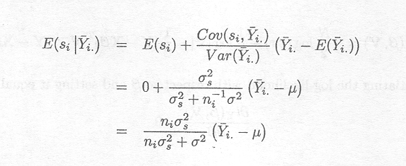
It can be shown (see Appendix D), given this joint distribution, that
As s2 tends to zero or
ni s![]() tends to infinity, this expression is approximately equal to (Yi, . µ). Otherwise,
the expression requires REML-estimates of the variance components and the
ML-estimate of µ, in order to obtain an estimate
i. As will be
shown in the next section, the ML-estimator for µ
can be obtained by
tends to infinity, this expression is approximately equal to (Yi, . µ). Otherwise,
the expression requires REML-estimates of the variance components and the
ML-estimate of µ, in order to obtain an estimate
i. As will be
shown in the next section, the ML-estimator for µ
can be obtained by

The random effects model presented above is fitted to
the data of Example 1.2.7. The REML estimates for the variance components are
given by s![]() = 3.685 and s2 = 3.542. The ML-estimate of the mean µ is given by
= 3.685 and s2 = 3.542. The ML-estimate of the mean µ is given by

The best linear unbiased prediction for the random effect of sire 4 is thus given by

The best linear unbiased predictions for the 8 sires in the data set can be obtained by the SAS program shown in Appendix B.2.3
Estimates of the fixed effects can be obtained by maximising the log-likelihood of Y

Differentiating the log-likelihood with respect to and setting it equal to 0

If the variance components contained in V are known and can be substituted into the expression, this estimator is called the generalised least squares estimator.
The variance-covariance matrix of ß is given by

However, the variance components contained in V are usually not known. Therefore, the REML-estimates need to be substituted, giving the estimate V, and the estimate based on the maximum likelihood criterion can then be obtained by the expression
= (XTV. 1X). XTV. 1Y
Furthermore, D(![]() ) is estimated by (XT
) is estimated by (XT![]() .
1X) . XT
.
1X) . XT ![]() .
1X (XT
.
1X (XT![]() . 1X) . This estimator is
biased downwards (i.e. is on the average smaller than the population value (XTV. 1X) . XTV . 1X (XTV. 1X) . ) since the uncertainty introduced with the
REML-estimates of the variance components in V is
not taken into account in the approximation for (XTV. 1X) (Kackar and
Harville,l984).
. 1X) . This estimator is
biased downwards (i.e. is on the average smaller than the population value (XTV. 1X) . XTV . 1X (XTV. 1X) . ) since the uncertainty introduced with the
REML-estimates of the variance components in V is
not taken into account in the approximation for (XTV. 1X) (Kackar and
Harville,l984).
We revisit Example 1.2.5. The mixed model is given by
Yijk = µ + di + rj + hij + Tk + (dT)ik +eijk
Since the model is overparameterised, the solution for ß is not unique; there exist an infinite number of solutions (see Section 2.2). This can also be seen by the fact that the matrix XTV . 1X is not of full rank and that we thus have to use generalised inverses. One solution is to set some of the parameter levels equal to 0, thereby reducing the number of parameter levels. In this example, the following restrictions are used
d2 = 0; T2 = 0; (dT )12 = 0; (dT)21 = 0;(d)22= 0
Therefore, a maximum likelihood estimate of the parameter vector
ßT = (µ, d1, d2, T1, T2, (dT)11, (dT)12, (dT)21, (dT)22)
can be shown, following substitution of ![]() for V, to
be
for V, to
be
![]() T = (17.13, 7.15, 0, 4.35, 0, . 3.18,
0, 0, 0)
T = (17.13, 7.15, 0, 4.35, 0, . 3.18,
0, 0, 0)
and the variance-covariance matrix
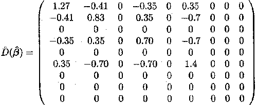
These results can be obtained by the SAS program shown in Appendix B.2.4.
Interest is not in the individual parameters of an overparameterised model (as they are not estimable), but in estimable functions of those parameters cTß so that the solution is independent of the generalised inverse. A simple example of such an estimable function is the mean of one level of a parameter (e.g. a treatment) averaged over other parameter levels. Both the estimate and the variance of the estimate of a linear combination of the parameters can easily be obtained if the vector of parameter estimates and its estimated variance-covariance matrix are available.
Assume that cTß is an estimable function. It is easy to show that the maximum likelihood estimator of cTß is given by cTß; the estimated variance (see Appendix E) is

As already mentioned, the cell means, being linear combinations of the parameters, are relevant and estimable parameters. In Example 1.2.5 the expected value for the first cell mean is given by the following linear combination
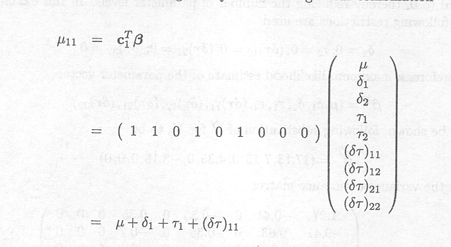
It represents the mean response of animals treated with a high dose of Berenil.
With c![]() = ( 1 0 1 0 1 0 0 0 1 ) we
obtain
= ( 1 0 1 0 1 0 0 0 1 ) we
obtain
This cell mean represents the mean response of animals treated with the low dose of Samorin.
Estimates for the cell means are then obtained by substituting the parameter
estimates obtained in Example 2.5.1.1

The variance of a cell mean ![]() 11 can also be
obtained.
11 can also be
obtained.
For instance, the estimated variance of ![]() 11 is given by
11 is given by
Vâr(c![]() = c
= c![]()
![]() (
(![]() )c1=1.27
)c1=1.27
This shows that the estimates for the cell means model can easily be obtained from the analysis of the overparameterised model. The SAS program that derives the cell mean estimates with their estimated variances is shown in Appendix B.2.5.
We often like to determine an upper and lower confidence
limit for an estimable parameter, say cTß.. Confidence intervals provide an appropriate
probabilistic tool for this. It leads to the determination of a lower and an
upper confidence limit for the parameter function under consideration. The
distributional properties of a specific linear combination, needed to derive
confidence intervals, follows easily from the fact that the estimators are
linear combinations of the observations Y. Since Y is multivariate normal,. the estimator cT![]() also follows a normal
distribution.
also follows a normal
distribution.
cT
~ N(cT, cTß, cT (XT V. 1 X) . c)
In general, however, the variance components in V must be estimated. So cT![]() is assumed to follow a t-distribution with v degrees of freedom, where v corresponds to the degrees of freedom available to
estimate the variance cT (XT V. 1X) _ c.
is assumed to follow a t-distribution with v degrees of freedom, where v corresponds to the degrees of freedom available to
estimate the variance cT (XT V. 1X) _ c.
In some situations, the calculated variance corresponds to the expected mean square of one of the random effects factors. In this case, the degrees of freedom are the degrees of freedom of the mean square itself, which can easily be determined (see Example 2.5.3.1).
In general in a mixed model, however, the variance of a linear combination is a complicated expression of different expected mean squares, and the degrees of freedom can only be approximated.
The Satterthwaite procedure (Satterthwaite, 1946), based on quadratic forms (mean squares typically are quadratic forms), provides a way to obtain approximate degrees of freedom and is given by

In this expression, the variance term in the denominator must be estimated. An approximation for this variance term has been proposed by Giesbrecht and Burns (1985) and McLean and Sanders (1988). The derivation of both the expression for the degrees of freedom and the approximation for the variance is discussed in detail in Appendix F.
If cT (XTV. 1X). c can be written as a linear combination of mean squares, i.e. a1MS1 +...+ a1MSl with al, ..., al constants and MSj the mean square due to the jth source of variation in the analysis of variance, then the Satterthwaite procedure simplifies to give

with dfj the degrees of freedom for MSj.
The (1 - a)100% confidence interval for cTß is then given by

Example 2.5.3.1 Confidence intervals
In the analysis of the data of Example 1.2.5, different linear combinations might be of
interest. Two linear combinations c![]() ß ~ and c
ß ~ and c![]() ß
have already been shown in Section 2.5.2.
ß
have already been shown in Section 2.5.2.
If the parameter vector is given by
ßT = ( µ d1 d2 T1 T2 (dT)11 (dT)12 (dT)21 (dT)22 )
some other examples of linear combinations are
1. The mean response for animals treated with Samorin, µ2,, given by
c![]() ß = ( 1 0 1 0.5 0.5 0 0 0.5
0.5) ß
ß = ( 1 0 1 0.5 0.5 0 0 0.5
0.5) ß
2. The mean difference between animals treated with Samorin and Berenil, µ2 . µ1., given by
c
ß = (0 -1 1 0 0 -0.5 -0.5 0.5 0.5) ß
3. The mean response for animals treated with a high dose of Samorin, µ21, given by
c
ß = ( 1 0 1 1 0 0 0 1 0) ß
4. The mean difference between animals treated with a high versus a low dose of Samorin, µ21 . µ22, given by
c
ß= (0 0 0 1 . 1 0 0 1 . 1 ) ß
It can easily be shown that an estimate for c![]() ß
is given by c
ß
is given by c![]() ß=
ß=
![]() 2.., with
2.., with ![]() 2..
the mean of the 12 observations on Samorin.
The corresponding variance is
2..
the mean of the 12 observations on Samorin.
The corresponding variance is
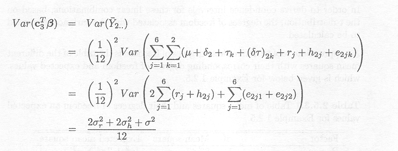
Similarly, variances for the other linear combinations can be obtained and are given by
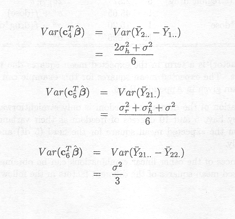
By substituting the REML-estimates of the variance
components (![]()
![]() = 5.15;
= 5.15; ![]()
![]() = 0.387;
= 0.387; ![]() 2 = 2.096) in these expressions, the following
estimates for the variances of the linear combinations are obtained
2 = 2.096) in these expressions, the following
estimates for the variances of the linear combinations are obtained
Vâr(c![]()
![]() ) = 1.0975
) = 1.0975
Vâr(c![]()
![]() )
= 0.478
)
= 0.478
Vâr(c![]()
![]() ) = 1.272
) = 1.272
Vâr(c![]()
![]() ) = 0.698
) = 0.698
In order to derive confidence intervals for these linear combinations, based on the t-distribution, the degrees of freedom associated with the variance term need to be calculated.
An appropriate tool to derive these degrees of freedom is the table of the different mean squares with their corresponding degrees of freedom and expected values, which is given below for Example 1.2.5.
Table 2.5.3.1. Table of mean squares and their degrees of freedom an expected values foe Example 1.2.5
|
Factor |
df |
Mean square |
Expected mean square |
|
Region |
5 |
23.47 |
4s |
|
Drug |
1 |
185.37 |
2s |
|
Herd (=region*drug) |
5 |
2.87 |
2s |
|
Dose |
1 |
45.65 |
s2 + f (dose) |
|
Drug*dose |
1 |
15.20 |
s2 + f (drug*dose) |
|
Error |
10 |
2.096 |
s2 |
where f (factor) is a term in the expected mean squares due to an individual fixed effect. The expected mean squares for this example can be obtained by the program given in Appendix B.2.6.
The derivation of the degrees of freedom is only
straightforward for c![]() ß and
c
ß and
c![]() ß. They have 5 and 10 degrees of freedom as their
variances are only dependent on the expected mean square for the herd (5 df) and
error (10 df), respectively.
ß. They have 5 and 10 degrees of freedom as their
variances are only dependent on the expected mean square for the herd (5 df) and
error (10 df), respectively.
The variances of the other linear combinations can be obtained by combining the expected mean squares of the different factors in the following way.
The variance of c![]() =
=![]() is (2s
is (2s![]() + 2s
+ 2s![]() + s2)/12. The numerator can be obtained from 0.5E(MSregion)+0.5E(MSherd).
Using the simplified Satterthwaite formula, with al
= a2 = 0.5, we obtain
+ s2)/12. The numerator can be obtained from 0.5E(MSregion)+0.5E(MSherd).
Using the simplified Satterthwaite formula, with al
= a2 = 0.5, we obtain

For c![]()
![]() . the variance is (s
. the variance is (s![]() + s
+ s![]() + s2)/16; the numerator can be obtained from
+ s2)/16; the numerator can be obtained from
0.25E(MSregion)+0.25E(MSherd)+0.5E(MSerror). Therefore

Thus, 95% confidence intervals are given by
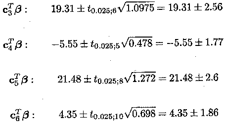
From these confidence intervals, it can be concluded
that there is a large and significant difference between animals treated with
Samorin and Berenil (c![]() ß.).
There is, however, no difference between the high and low dose of Samorin (c
ß.).
There is, however, no difference between the high and low dose of Samorin (c![]() ß.). These estimates and their standard errors can be
obtained by the SAS program given in Appendix B.2.7.
ß.). These estimates and their standard errors can be
obtained by the SAS program given in Appendix B.2.7.
From the example in the previous section it is clear that the variance of cTß. with cTß. estimable, is a linear combination of the variance components present in the mixed model. In some situations it is meaningful to narrow the scope of the study and to think about one or more of the random effects as fixed effects. As a consequence, the corresponding variance components will not appear in the expression of the variance for the estimator cTß.. If we think of one or more of the random effects as fixed effects we say that we consider a narrow inference space. If we assume all effects to be random we talk about the broad inference space. Based on examples we show that the confidence limits for cTß. are quite different for broad and narrow inference spaces. If we consider all factors as fixed effects the only variance component is s2, the error term variance. It typically follows that the narrower the inference space the smaller will the confidence interval be.
It has been shown for the data of Example 1.2.5 that the variance of the mean response of animals treated with Samorin, µ2, is given by
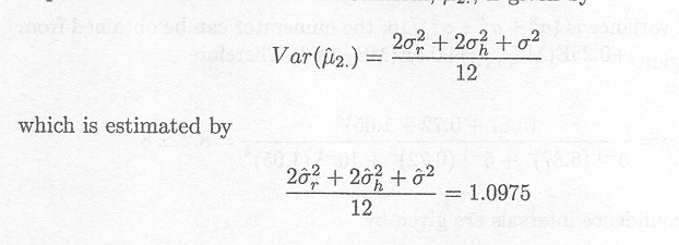
The variance of ![]() 2 ...,
the estimate of µ2,
in the fixed effects model, i.e., the model with region and herd as fixed
effects, is
2 ...,
the estimate of µ2,
in the fixed effects model, i.e., the model with region and herd as fixed
effects, is
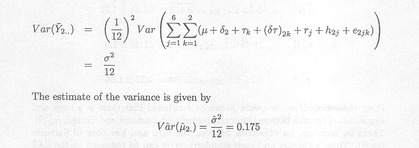
This estimate is much smaller than that calculated
previously for c![]() ß.
when rj and h2j are assumed random,
and therefore the width of the confidence interval for µ2. is much
narrower.
ß.
when rj and h2j are assumed random,
and therefore the width of the confidence interval for µ2. is much
narrower.
The estimated standard errors for the linear combination µ2, can be obtained by the SAS program given in Appendix B.2.8 for both the fixed effects model and the mixed model.
Testing general linear hypotheses for fixed effects by an appropriate F-test is much more complex in mixed models than in fixed effects models. As has already been shown, there is only one source of random variation in fixed effects models. The F-statistic consists of a ratio of two mean squares, the denominator being the error mean square. For that reason the derivation of the degrees of freedom of the denominator of the F-test is straightforward, as shown before. In the mixed model, however, there are different sources of random variation, and the denominator of the F-test consists in most cases of a combination of these different sources of random variation. The derivation of the appropriate degrees of freedom for the denominator in the F-test is therefore not straightforward, and can, in most practical cases, only be approximated by the Satterthwaite procedure as described in Appendix F.
General linear hypotheses for the fixed effects take the form
H0 : CTß. = 0 versus Ha : CTß.? 0
with ß a (b x 1) vector and C a (b x q) matrix of vi independent and estimable functions. Thus (rank(C)=vl).
To estimate CTß we use CTß and since
D(CTß) = CT D(ß)C = CT (XT V . 1X) .C
we use CT (XT V . 1X) . C as the estimated variance-covariance matrix.
It can be shown that the statistic

approximately follows a F-distribution under the null hypothesis with v1 as numerator degrees of freedom.
As can be seen from this expression, F is no longer a ratio of two mean squares as in the fixed effects model. The role of the denominator is taken over by (XTV. 1X). The denominator degrees of freedom, v2, thus correspond to the degrees of freedom associated with (XTV. 1X) and can be approximated by the Satterthwaite procedure in a similar way as shown for the t-test. Further details on these approximate F-tests for general linear hypotheses are in Fai and Cornelius (1996).
The P-value for testing the null hypothesis is then given by the probability that Fv1, v2 is larger than the corresponding value of the F-distribution, i.e.
Prob (Fv1,v2 = F)
The null hypothesis and alternative hypothesis of no difference between Samorin and Berenil in Example 1.2.5 are given by
H0 : µ2. = µ1. and Ha : µ2 ? µ1.
Thus in this simple case, where C is a (q x 1) vector, the null hypothesis CTß = 0
can be written as
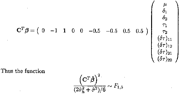
follows a F-distribution with 1 and 5 degrees of freedom
(with 5 being the degrees of freedom associated with region as calculated before
for c![]() ß). The estimate for CTß equals . 5.55 and an estimate for its variance is
given by 0.478.
ß). The estimate for CTß equals . 5.55 and an estimate for its variance is
given by 0.478.
Therefore, the P-value for the null hypothesis is given by

In testing a more complex hypothesis in which C is a matrix rather than a vector, assume that, for Example 1.2.5, interest is in the following hypothesis
H0 : µ11 = µ12 = µ21 = µ22 versus Ha : not all µij equal
We can rewrite this hypothesis by building up three simultaneous independent estimable functions and testing them together

The first estimable function tests whether there is a difference between drugs (=µ1. . µ2.), the second between doses (=µ.1 . µ.2) and the third whether there is an interaction between dose and drug (=(µ11. µ12) . (µ21 . µ22)).
It can be shown that the value of the F-statistic is 31.2 and that the denominator degrees of freedom equal 7.14. The rank of C and thus the numerator degrees of freedom equal 3. Therefore, the P-value is Prob(F3,7 = 31.2) = 0.0002. The null hypothesis is clearly rejected. The corresponding SAS program is given in Appendix B.2.9.