Chapter 3

Into the realm of mixed models

3.1 Introduction

3.2 Designed experiments. Example 3.1

3.3 Mixed models with emphasis on random effects. Example 3.2

3.4 Covariance structures in the mixed model. Example 3.3

3.1 Introduction

The mixed model methodology has been developed within the discipline of animal genetics and breeding (Henderson, 1990). From there, it has spread to many other disciplines, and mixed models have been fitted and used for analysis of various types of data. Many applications in veterinary science are based on mixed rather than fixed effects models.

In this chapter three diverse situations will be described where the appropriate statistical analysis is based on mixed models techniques.

The first field, discussed in Section 3.2, is that of designed experiments, such as randomised complete block, split-plot and latin square designs. In these experiments block parameters may be best described by variance components which describe the background variability against which different hypotheses are tested.

The second field, discussed in Section 3.3, is that of experiments for which there is primary interest in both random and fixed effects. Experiments in this field include breeding experiments (Gianola and Hammond, 1990) and epidemiological studies.

The third field, discussed in Section 3.4, is that of experiments in which observations are correlated with each other, either because they are repeated measurements in time (Diggle et al., 1994) or because they are spatially correlated (Cressie, 1991; Ripley, I981). For such experiments interest is in the fixed effects as well as in the types of correlations among observations.

An experiment can of course consist of a combination of these three categories. For instance, a designed experiment might also have repeated measures, for which the correlation structure must be determined. The three categories will, however, be explained separately in order to focus on the important concepts.

The data are given in Appendix A and the full SAS programs in Appendix B. Relevant information extracted from the SAS output of the programs is shown in this chapter.

3.2 Designed experiments. Example 3.1

To demonstrate how the mixed model can be used for designed experiments, the following experiment is analysed by the mixed model.

Two drugs against trypanosomosis, Berenil and Samorin, are studied in a situation where there is widespread evidence of high levels of drug resistance. Four herds of cattle are randomly assigned to Berenil and four herds to Samorin treatment. It was considered impracticable to organise the study so that both drugs were used in the same herd. Only one dose of Samorin (comparable with the low dose of Berenil) is used. Animals belonging to a herd to which Berenil has been assigned, however, are randomly assigned to receive a high or a low dose of Berenil when detected parasitaemic with trypanosomes.

Packed cell volume was monitored monthly. That determined at the time of treatment was designated PCVl, that a month later following treatment was designated PCV2. A significant increase in PCV reflects a beneficial effect of treatment, despite presence of drug resistance. The data are shown in Appendix A, Example 3.1.

Different models can be fitted to this data structure and three different models with different degrees of complexity are fitted here.

Model 1

In the first model the data structure can be described by

Y_ijkl = µ + T_i + h_ij + δ_ik + e_ijkl

where, for i = 1, 2; j = 1, 2, 3, 4; k = 1, 2 if i = 1; k = 1 if i = 2; l = 1, ..., n_ijk,

Y_ijkl is the PCV one month after drug administration (=PCV₂)

µ is the overall mean

T_i is the effect of Berenil (T_l) or Samorin (T₂)

h_ij is the effect of herd j to which drug i is assigned

δik is the effect of the low (δ₁₁) or high (δ₁₂) dose of Berenil or the low (δ₂₁) dose of Samorin

e_ijkl is the random error of animal l with dose k of drug i in herd ij

Each of µ, T_i and δ_ik are fixed effects; h_ij and e_ijkl are random effects.

The assumptions are:

the h_ij are iid N(0, σ)

the e_ijkl are iid N(0,σ ²)

h_ij and e_ijkl are independent

In this model, the information on PCV at the time of treatment is not used. The SAS-program that fits this model is shown in Appendix B.3.1.1. The REML-estimates of the variance components can be obtained from the 'Covariance Parameter Estimates (REML)' table:

Covariance Parameter Estimates (REML)
Cov Parm	Estimate
HERD	0.2572
Residual	15.4001

The variance component describing the variability among animals in the same herd is much larger than that among herds. Thus in this example there is little additional variability among animals from different herds compared with animals from the same herd.

Once estimates of the variance components have been obtained, they can be used to derive estimates of the fixed effects. These estimates can be obtained from the 'Solution for Fixed Effects' table.

The model, as described above, is overparameterised, and a solution is thus obtained by ensuring that functions of parameters are estimable. SAS does this by setting some parameter levels to 0. In the solution supplied by SAS, the following parameters are set to 0.

T₂ = 0; δ₁₂ = 0; δ₂₁ = 0

Therefore, INTERCEPT in the table is the expected value of PCV2 for any animal l in any herd j treated with the one dose of Samorin and is given by

E(PCV2_2j1l) = 23.89

The expected values of PCV2 for the three treatments are shown in the 'Least Squares Means' table:

Least Squares Means
Effect	DRUG	DOSE	LSMEAN	Std Error	DF	t	Pr > ½t½
DOSE(DRUG)	BERENIL	1	23.31	0.45	8.24	51.84	0.0001
DOSE(DRUG)	BERENIL	2	23.96	0.46	9.69	52.13	0.0001
DOSE(DRUG)	SAMORIN	1	23.89	0.44	7.28	54.03	0.0001

Note that the value 23.89 in the third line is the same as the INTERCEPT described above. The classical hypotheses tests for the fixed effects can be obtained from the 'Tests of Fixed Effects' table. These are based on the F-distribution and the denominator degrees of freedom (DDF) of the F-statistic is obtained by the Satterthwaite procedure.

Taste of Fixed Effects
Source	NDF	DDF	Type III F	Pr > F
DRUG	1	5.56	0.2	0.674
DOSE(DRUG)	1	348	1.49	0.224

NDF refers to the degrees of freedom of the numerator of the F-test; type III F means that the hypothesis being tested is that corrected for the other effects in the model. The first line, DRUG, tests whether there is a difference in the response to the two drugs; the obtained F-value is not significant. The second test compares the two doses of Berenil, and again no significant difference is found. Note the large difference in DDF, denominator degrees of freedom, for the two tests. This is because the alternative drugs are assigned to the herds as a whole, and therefore the comparison between drugs is based on differences between herds, of which there are only eight in the study. On the other hand, the comparison of the two doses of Berenil is based on animals within herds.

Often our interest is in more specific hypotheses than the general ones just described above. Any linear hypothesis can be tested by specifying the hypothesis as a linear combination c^Tβ = 0 or set of linear combinations C^Tβ = 0.

We might want to test whether a similar dose of Berenil and Samorin leads to the same response in PCV. This hypothesis is not included in the 'Tests of Fixed Effects' table. The hypothesis of interest can be written as:

H₀ : µ₁₁ = µ₂₁ versus H_a : µ_11≠ µ₂₁

The null hypothesis can be rewritten as the following linear combination

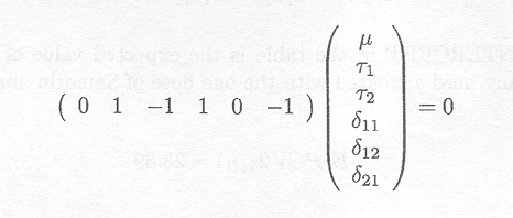
An estimate of this linear combination can be obtained from the third line in the 'ESTIMATE Statement Results' table.

ESTIMATE Statement Results
Parameter	Estimate	Std Error	DIP	t	Pr > ½t½
Mann Samorin	23.89	0.442	7.28	54.03	0.0001
Berenil dif 2 doses	– 0.644	0.628	348	–1.22	0.224
Bar va Sam at dose 1	–0.578	0.831	7.75	– 0.92	0.387

As expected, there is no significant difference between Berenil and Samorin when given in similar doses. The estimated difference is only . 0.578, which is of the same level of magnitude as the standard error which equals 0.631.

The hypotheses present in the 'Tests of Fixed Effects' table can also be tested by rewriting them in terms of appropriate contrasts. For instance, testing whether the two doses of Berenil lead to the same response can be done by testing the hypothesis

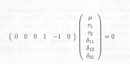
and this leads, as shown in the second line of the 'CONTRAST Statement Results' table, to the same test as the one described in the 'Tests of Fixed Effects' table.

CONTRAST Statement Results
Source	NDF	DDF	F	Pr > F
Mean Samorin	1	7.28	2919.6	0.0001
Berenil dif 2 doses	1	348	1.49	0.224
Ber vs Sam at dose 1	1	7.75	0.84	0.387
Some difference	2	21.1	0.85	0.52

Furthermore, means can be estimated by specifying the appropriate linear combination. For instance, the mean PCV for Samorin can be obtained by estimating

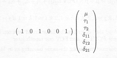
which leads to the same results as shown before in the 'Least Squares Means' table.

Finally, more complex hypotheses can be tested, consisting of different independent linear combinations.

If we want to test whether there exists any genuine difference between the three treatments, expressed as

H₀ : µ₁₁ =µ₁₂ = µ₂₁ versus H_a : µ_ik s are not equal

 it can be translated as

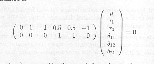
Note that these two linear combinations are independent as their vector product equals 0. The first combination tests whether there is a difference between the two drugs, averaging the response for the high and the low dose for Berenil, whereas the second linear combination tests whether there is a difference between the low and the high dose of Berenil. As we have three treatment means, testing any two independent linear combinations simultaneously corresponds to testing the above hypothesis.

The actual F-value for this hypothesis testing problem is shown in the last line of the 'CONTRAST Statement Results' table, and again, as expected, the null hypothesis is not rejected.

Model 2

Information on the PCV of the animals at the time of treatment is not used in the above analysis. The analysis might be made more powerful if this is used. We indeed expect that animals with very low PCV at the time of treatment may benefit more from the administration of the drug and demonstrate a higher increase in PCV. In order to analyse this type of response the following model is fitted

Y_ijkl = µ +β x (PCV1_ijkl) + T_i + h_ij + δ_ik + e_ijkl

 where, for i = 1, 2; j = 1, 2, 3, 4; k = 1, 2 if i = l; k = 1 if i = 2; l = 1, ..., n_ijk,

β is the slope that describes the linear trend between PCV at time of treatment PCV1_ijkl and PCV one month later

all other parameters having the same meaning as in Model 1.

The SAS program that fits this model is shown in Appendix B.3.L2.

Estimates for the parameters can be obtained again from the 'Solution for Fixed Effects' table.

It follows from this table that there is indeed a significant effect of the PCV measured at the time of treatment on the PCV one month after treatment. The effect of initial PCV on the response variable can be separately determined for each treatment group. For instance, for the animals treated with the low dose of Berenil, this relationship is given by

E(Y_1j1l½PCV1_1j1l = x ) = 18.548 + 0.266x + 0.249 - 0.687

= 18.11 + 0.266x

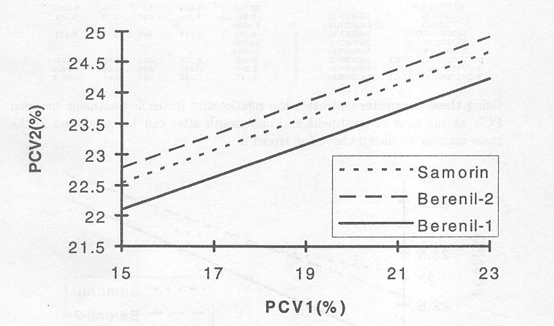
Figure 3.2.1 The effect of initial PCV on PCV one month after treatment for the three treatments based on Model 2.

Although Figure 3.2.1 indicates that the regression line for the lower dose of Berenil falls below the other two, the 'Solution for Fixed Effects' table above indicates no significant mean differences between treatments. Thus, whereas the increase in PCV is greater for lower PCV1, responses were overall similar for each treatment.

Model 3

In Model 2, three regression lines with the same slope were fitted for the three treatments to relate PCV2 to PCVl. Now we relax this assumption and fit a model that allows a different slope for each treatment group. This leads to the following model

Y_jkl = µ + β_ik x (PCV1_ijkl ) + T_i + h_ij + δ_ik + e_ijkl

 where, for i =1, 2; j = 1, 2, 3, 4; k = 1, 2 if i = l; k = 1 if i = 2; l = 1, ..., n_ijk,

β_ik is the fixed effect of PCVl at time of treatment on PCV one month later for dose k of drug i

all other parameters having the same meaning as in Model 1

The SAS program that fits this model is shown in Appendix B.3.1.3. Estimates for the parameters can be obtained again from the 'Solution for Fixed Effects' table.

Solution for Fixed Effects
Effect	DRUG	DOSE	Estimate	Std Error	DF	t	Pr > ½t½
INTERCEPT			20.733	3.264	328	6.35	0.0001
DRUG	BERENIL		– 2.554	4.344	332	– 0.59	0.557
DRUG	SAMORIN		0.0000
DOSE(DRUG)	BERENIL	I	– 2.019	4.744	343	– 0.43	0.671
DOSE(DRUG)	BERENIL	2	0.0000
DOSE(DRUG)	SAMORIN	I	0.0000
PCVl*DOSE(DRUG)	BERENIL	1	0.366	0.193	342	1.90	0.0588
PCVl*D03E(DRUG)	BERENIL	2	0.298	0.146	345	2.04	0.0424
PCVl*DOSE(DRUG)	SAMORIN	1	0.157	0.161	344	0.97	0.3325

Using these parameter estimates the relationship for each treatment between PCV at the time of treatment and one month after can be calculated in the same manner as shown above for Model 2.

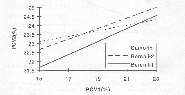
Figure 3.2.2 The effect of initial PCV on PCV one month after treatment for the three treatments based on Model 3.

The figure shows that, whichever treatment is used, the higher the PCV at the time of treatment, the lower its increase in response to treatment. On the other hand, when PCVl was low both Samorin and Berenil at the high dose appeared to result in higher increases in PCV1 than Berenil at the low dose. The 'Solution for Fixed Effects' table demonstrates that the slope for Samorin is not significant.

An investigator might be interested in estimating how an animal might benefit from the treatment for different values of PCV. This might lead to a recommendation on the value to which PCV needs to fall before treatment should be administered. For a value of PCVl=x, the expected response in PCV for drug i at dose k is given by

E(Y_jkl /PCV1_ijkl = x) = µ + β_iikx + T_i + δ_ik

An estimate for PCV for animals with PCVl=18 % at time of treatment with the low dose of Berenil, for instance, is given by:

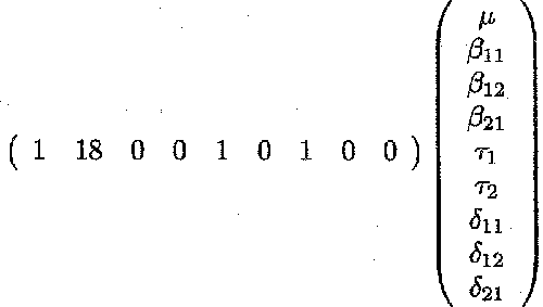
Estimates for PCV1=18 can be obtained from the 'Least Squares Means' table.

A 95% confidence interval for the mean PCV of animals treated with the low dose of Berenil is then given by

22.74 ± t_{0.025; 20} x 0.52 = 22.74 ± 1.08

Thus an effective increase in PCV of 4.74 ± 1.08% would have occurred as a result of treating animals with a PCV of 18%.

3.3 Mixed models with emphasis on random effects. Example 3.2

The emphasis in breeding experiments is on the variance components and on the prediction of particular random effects, but estimation of fixed effects and hypothesis testing with regard to fixed effects is also important. In epidemiological studies both random and fixed effects may be of interest.

An animal breeding experiment is used to illustrate this. A portion of the data set is shown in Appendix A, Example 3.2. The goal of the research is to select for improved helminth resistance in sheep. The female sheep used in the experiment are from three different breeds, whereas the males are from two breeds. In each of the six crosses, there are at least 25 and at most 42 different sires, and each sire within a cross breed has on average offspring of 6.4 lambs. The weaning weight is measured for each of the lambs. The age at which lambs are weaned (AGEW) may differ from animal to animal, and therefore, a variable expressing the age of the animal at weaning is included as a fixed effect in the model. Also the sex (SEX) of the lamb is added to the model as a fixed effect. Finally, the sire is included as a random effect: Although the same sire is mated to ewes from different breeds, the sire nested in breed is taken as a single random effect and it is assumed that these random effects are independent.

An appropriate model for this data structure is thus given by

Y_ijkl = µ + y_i + s_ij + T_k + β (AGEW) + e_ijl

where, for i = 1, ..., 6; j = 1, ..., n_i; k = 1, 2; l = 1, ..., nij;

Y_ijkl is the weaning weight of lamb l of sex k from sire j within breed i

µ is the overall mean

y_i is the effect of breed i

s_ij is the effect of sire j within breed i

T_k 1S the effect of sex: female (T₁) or male (T₂)

β is the effect of age at weaning on weaning weight

e_ijl is the random error of lamb l from sire j within breed i

Each of µ,β , y_i and T_k are fixed effects, whereas s_ij and e_ijl are random effects with the following assumptions:

the s_ij are iid N(0, σ)

the e_ijl are iid N(0,σ ²)

s_ij and e_ijl are independent

The SAS-program that fits this model is given in Appendix B.3.2. The REML-estimates of the variance components can be obtained from the 'Covariance Parameter Estimates (REML)' table.

A commonly derived statistic is the heritability (h²) of the trait, which is a function of these two variance components and describes the proportion of the total variation in the environment of this study attributable to inheritance from the lambs' parents.

In this formula is multiplied by 4 in the numerator to account for the fact that lambs from the same sire are half siblings and the sire accounts for half of the inherited genetic component, and (+ ²) is the phenotypic variance. The higher the heritability, which lies between 0 and 1, the higher the proportion of total variation that can be assumed to be genetic.

Once estimates of the variance components have been obtained, they can be used to derive estimates of the fixed effects. These estimates can be obtained from the 'Solution for Fixed Effects' table.

There is a significant effect of sex with female lambs weighing on average 0.704 kg less at weaning than males. Furthermore, there is a significant effect of age at weaning with weaning weight increasing by 0.046 kg per daily increase in age. There are also significant differences among breeds, with breeds 1– 4 having significantly higher weaning weights than breeds 5– 6. Breed means axe given in the 'Least Squares Means' table.

Least Squares Means
Effect	BREED	LSMEAN	Std Error	DF	t	Pr >½t½
BREED	1	12.48	0.222	216	56.23	0.0001
BREED	2	12.31	0.232	170	53.00	0.0001
BREED	3	12.23	0.187	145	65.21	0.0001
BREED	4	11.75	0.187	102	62.79	0.0001
BREED	5	10.39	0.249	160	41.70	0.0001
BREED	6	10.80	0.304	420	35.54	0.0001

To compare these means we can use a multiple comparisons procedure, such as Tukey-Kramer (see SAS Institute Inc. Cary, NC, 1996 on the procedure MULTTEST and Westfall and Young, 1993). The results are given in the underlying 'Differences of Least Squares Means' table. Some of the columns of the original table have been deleted.

Differences of Least Squares Means
Effect	BREED	_BREED	Difference	Std Error	Adj. P
BREED	1	2	0.166	0.321	0.995
BREED	1	3	0.246	0.291	0.958
BREED	1	4	0.733	0.290	0.122
BREED	1	5	2.088	0.334	0.000
BREED	1	6	1.682	0.376	0.000
BREED	2	3	0.079	0.299	0.999
BREED	2	4	0.567	0.298	0.406
BREED	2	5	1.921	0.342	0.000
BREED	2	6	1.515	0.382	0.001
BREED	3	4	0.487	0.265	0.443
BREED	3	5	1.842	0.312	0.000
BREED	3	6	1.436	0.357	0.001
BREED	4	5	1.354	0.312	0.000
BREED	4	6	0.948	0.357	0.089
BREED	5	6	–0.406	0.393	0.906

From this table, it can be concluded that significant differences exist when comparing breed 1, 2, 3 and 4 with breed 5 and 6, but not among 1, 2, 3 and 4 nor among 5 and 6.

Apart from estimating heritability and comparing breed means, an investigator might be interested in the breeding value of specific sires in order to determine which sires should be retained for future selection. As seen before, such a prediction of the breeding value of a sire can be obtained by best linear unbiased prediction. For each sire, such a prediction can be obtained from the 'Solution for Random Effects' table.

Effect	SIRE-ID	BREED	Estimate	SE Pred	DF	t	Pr >½t½
SIRE_ID(BREED)	1971	1	–0.1061	0.6653	85.9	–0.16	0.874
SIRE-ID(BREED)	1972	1	0.5241	0.5349	189	0.98	0.328
SIRE_ID(BREED)	1973	1	0.3888	0.6399	99.9	0.61	0.545
SIRE_ID(BREED)	1974	1	1.9339	0.5486	174	3.53	0.000

The predicted breeding value for sire with ID 1974 equals 1.93, meaning that offspring of this sire are predicted to have a weaning weight that is 1.93 kg higher than the average offspring of all sires of the same breed.

3.4 Covariance structures in the mixed model. Example 3.3

An important assumption in the use of the fixed effects model is that observations are independent from each other. In many practical situations this assumption may not hold. The most common situation is where different measurements are taken on the same individual, leading to what is known as a repeated measures design. Often these measurements are taken periodically over time. Alternatively, observations may be spatially collected in which case those closest together may be most alike.

As an example, we study the repeated measures design introduced in Example 1.2.8.

The aim of the study was to see whether there are differences in the change in PCV between the two breeds following a trypanosome infection. It is clear that observations collected over time on the same animal are correlated. The data set is shown in Appendix A, Example 3.3. Different models can be fitted to the data with different assumed covariance structures.

Model 1

The data structure can be described by the following statistical model

Y_ikl = µ + β_i0 +β _ilt_l +a_ik + e_ikl

where, for i = 1, 2; k = 1, ..., 6; l = 1, ...14

Y_ikl is the PCV of animal k of breed i at time l

µ is the overall mean

β_i0 is the intercept of the linear regression line for breed i

β_i1 is the slope of the linear regression line for breed i

t_l is the time of measurement l

a_ik is the effect of animal k belonging to breed i

e_ikl is the random error of measurement l on animal k of breed i

Both a_ik and e_ikl are random effects, independent from each other, with the assumptions

the _ik are iid N(0, σ)

the e_ikl are iid N(0,σ ²)

From this model structure, it follows that

We introduce a new notation, putting the suffix l of Y_ikl into brackets to clearly separate suffix k from suffix l which can consist of two numbers (l goes from 1 to 14). Thus Y_ikl = Y_ik(l).

Therefore, the covariance structure of the 14 observations Y_ik = (Y_ik(1), ..., Y_ik(14)) on the same animal, W = D(Y_ik), is given by

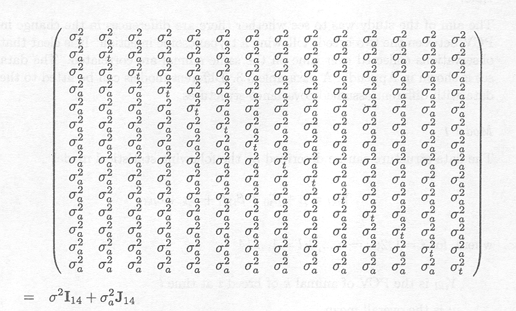
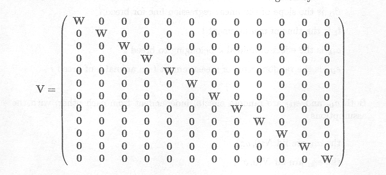
As measurements on different animals are independent from each other, the variance-covariance matrix of the observation vector Y is given by

An alternative model representation can thus be given by

Y_ikl = µ + β_i0 + βi_lt_l + e_ikl

where we drop the independence assumption on the e_ikl. The within-subject correlations, modelled by the random effects factor a_ik; in the first model representation, are now modelled by specifying a more complex variance-covariance matrix for e_ikl (=e_ik(l)).

For the random errors of an individual animal, e_ik =(e_ik(1), ..., e_ik(14)), is it now assumed that

e_ik ~ MVN(0, σ ²I₁₄ + σJ₁₄

and also that

D(e_ik) = D(Y_ik) and D(e) - D(Y) = V

This type of covariance structure is called compound symmetry with each observation on an animal having the same correlation with each other observation measured on the same animal.

The advantage of the first model specification is that it uses the general notation for the mixed model and it shows how the covariance structure can be expressed in terms of two random effects. The disadvantage of the first model specification is that it can only deal with the compound symmetry structure. If a more complex covariance structure is assumed, the second model specification needs to be used, as will be shown in Model 2.

The SAS-program that fits these two model specifications is given in Appendix B.3.3.1. Since the two model specifications lead to the same results, we only discuss here the results from the first model specification.

The REML-estimates of the variance components can be obtained from the 'Covariance Parameter Estimates (REML)' table.

Covariance Parameter Estimates (REML)
Cov Parm	Estimate
ANIM_ID(BREED)	5.478
Residual	4.965

The covariance parameter 'ANIM-ID(BREED)' equivalent to the variance component σ in the model corresponds to the covariance among measurements within an animal (see matrix D(Y_ik) above).

Based on these results, we can conclude that the estimated covariance between two measurements within the same animal is equal to 5.478, whereas the estimated variance of a single measurement (given by ^σ2+σ) is 5.478+4.965=10.443.

Estimates can be obtained from the 'Solution for Fixed Effects' table.

From this table, the linear changes in PCV of the two breeds with time can be obtained as

BO: PCV = 35.06 – 0.842 - 0.413t

ND: PCV = 35.06 - 0.276t

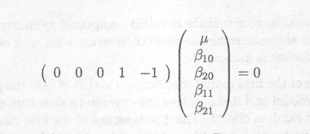
Thus, PCVs of the Borans appear to decrease more rapidly than those of the N'Damas. To determine whether this is statistically significant a contrast can be written

Alternatively, the model can be expressed in a different way with time as fixed effect and the time*breed term now representing the interaction between time and breed. The model can be written as

Y_ikl = µ + β_i0 + β₁t_l + β_i1t_l + e_ikl

where β_i1 now represents the difference in slope for breed i from the average.

The program fitting this model is given as the third mixed procedure statement in Appendix B.3.3.1. The significance test for this interaction can be found from the 'Tests of Fixed Effects' table.

Tests of Fixed Effects

Source	NDF	DDF	Type III F	Pr > F
TIME	1	154	470.06	0.0001
BREED	1	10	0.32	0.585
TIME-BREED	1	154	18.62	0.0001

This table shows that the rate of decrease is different for the two breeds as indicated by the significant interaction term. On the other hand, the intercept of the two lines do not differ significantly as shown by the F-test for breed.

The slopes for the two breeds are shown in the 'Solution for Fixed Effects' table above. These are fixed effects and assumed to be the same for each animal within a breed. However, having introduced a random animal effect into the model, a different intercept can be calculated for each animal. The intercept for a particular animal can be obtained from the 'Solution for Random Effects' table.

For instance, for the first animal, BO241, the fitted relationship is equal to

BO241 : PCV = 34.22 – 0.672 – 0.413t

               PCV = 33.55 – 0.413t

These relationships can be determined for each animal and are presented in the following figure

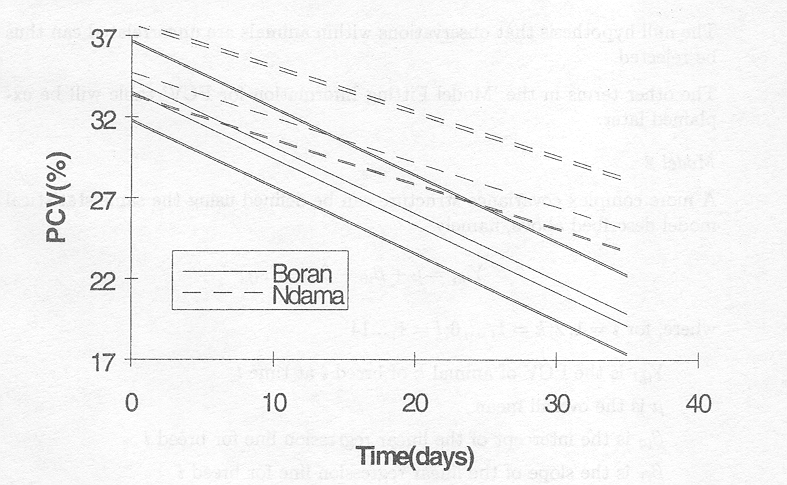
Figure 3.4.1 Change of PCV in time for individual animals based on Model 1. Bold dots and dashes indicate more than one animal with this line.

The second model specification leads to the same results, although the presentation of the results is somewhat different. An interesting additional feature in the output of the second model specification comes from the 'Model Fitting Information for PCV' table.

Model Fitting Information for PCV
Description	Value
Observations	168.000
Res Log Likelihood	– 391.73
Akaike's Information Criterion	– 393.73
Schwarz's Bayesian Criterion	– 396.83
-2 Ras Log Likelihood	783.451
Null Modal LRT Chi-Square	80.848
Null Model LRT DF	1.0000
Null Model LRT P-Value	0.0000

The last three lines contain the information that can be used to compare the suitability of the model with the compound symmetry covariance structure with that with the independent covariance structure (Null Model). As the compound symmetry covariance structure model is nested within the independent covariance structure model in the sense that the latter structure contains an additional term σ, the null hypothesis that the two models describe the data equally well can be tested via the likelihood ratio test (LRT), which equals 80.845. As the nested model contains one more parameter, the likelihood ratio statistic is asymptotically Chi-square distributed with one degree of freedom and the P-value is

Prob(X≥ 80.845) < 0.00001

The null hypothesis that observations within animals are uncorrelated can thus be rejected.

The other terms in the 'Model Fitting Information for PCV' table will be explained later.

Model 2

A more complex covariance structure can be defined using the same statistical model described above, namely

Y_ikl = µ +β_i0 +β_i1 t_l + e_ikl

where, for i = 1, 2; k = 1, ..., 6; l = 1, ...14

Yikl is the PCV of animal k of breed i at time l

µ is the overall mean

β_i0 is the intercept of the linear regression line for breed i

β_i1 is the slope of the linear regression line for breed i

t_l is the time of measurement l

e_ikl is the random error of measurement l on animal k of breed i

As before, the random error terms within animals are not assumed independent, but can now be defined to have another and more complex covariance structure. Such a more complex covariance structure D(e_ik) for the random error term is the first-order autoregressive structure given by

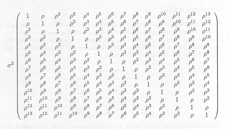
In this matrix, 0 < p < 1 represents the correlation between two observations adjacent in time. This way of modelling the covariance structure means that observations on the same animal that are further apart in time have smaller correlation. The SAS program that fits this model is given in Appendix B.3.3.2. The residual variance σ² and the correlation p can be obtained from the 'Covariance Parameter Estimates (REML)' table.

Covariance Parameter Estimates (REML)
Cov Parm	Subject	Estimate
AR(1)	ANIM_ID(BREED)	0.621
Residual		10.191

The estimate for σ² is 10.191 and the estimate for p is 0.621. The covariance between adjacent observations on the same individual is thus 0.621 x 10.191 = 6.33. The covariance between observations on the same animal decreases the more the observations are apart in time. For instance, the covariance between an observation at time 1 and time 5 or between an observation at time 2 and time 6 equals

Cov(Y_ik1Y_ik5) = Cov(Y_ik2, Y_ik6) = σ²p⁴

This covariance is estimated as ²⁴= 1.52.

T he covariance between an observation at time 1 and time 10 or between an observation at time 3 and time 13 equals

Cov(Y_ik1, Y_ik10) = Cov(Y_ik3, Y_ik13) = σ²p⁹

The estimate is 0.141.

To compare Model 1 and Model 2 we cannot use the likelihood ratio test since neither of these models are nested within each other. The models however do have the same number of parameters. We therefore choose a model with the higher value for the log-likelihood. This information can be obtained from the 'Model Fitting Information for PCV' table.

Model Fitting Information for PCV
Description	Value
Observations	168.000
Res Log Likelihood	–396.57
Akaike's Information Criterion	–398.57
Schwars's Bayesian Criterion	–401.67
-2 Res Log Likelihood	793.139
Null Model LRT Chi-Square	71.156
Null Model LRT DF	1.0000
Null Model LRT P-Value	0.0000

The restricted log-likelihood, which is the log-likelihood for an independent set of linear combinations KY as defined in Section 2.4.2, for this model is -396.57. In the corresponding table for the compound symmetry model the restricted log-likelihood equals –391.73. Thus the compound symmetry covariance structure has a slightly higher log-likelihood and thus describes the data better. In a similar way, other covariance structures can be fitted and compared. The two other criteria 'Akaike's Information Criterion' (Akaike, 1974) and 'Schwarz's Bayesian Criterion' (Schwarz, 1978) can also be used to compare models, especially if they contain different number of parameters. They are both based on the log-likelihood, but are penalised for the number of parameters estimated. The larger the value the better the model fits the data. In this case, with equal number of parameters for the two models, these alternative criteria lead to the same conclusion as the restricted log-likelihood.

Model 3

In Models 1 and 2, average slopes for the two breeds are fitted as fixed effects. Thus, the decreases in PCV with time are assumed to be parallel for all animals within a breed, i.e. the slope is the same. This assumption can be further relaxed by assuming that each animal has also a random slope, and that this random slope is normally distributed.

This random coefficients model (Longford, 1993) is given by

Y_ikl = µ +β_i0 + β_i1 t_l + a_ik + b_ikt_l + e_ikl

where, for i = 1, 2; k = 1, ..., 6; l = 1, ...14,

Y_ikl is the PCV of animal k of breed i at time l

µ is the overall mean

β_i0 is the intercept of the linear regression line for breed i

β_il is the slope of the linear regression line for breed i

a_ik is the random intercept of animal k of breed i

b_ik is the random slope of animal k of breed i

t_l is the time of measurement l

e_ikl is the random error of measurement l on animal k of breed i

Both a_ik, b_ik and e_ikl are random effects with the assumptions

the a_ik are iid N(0, σ)

the b_ik are iid N(0, σ)

the e_ikl are iid N(0,σ ²)

Moreover, we assume that both a_ik and b_ik are independent from e_ikl but that a_ik and b_ik are possibly correlated.

The program that fits this model is shown in Appendix B.3.3.3.

The variance components of the random effects factors can be obtained from the 'Covariance Parameter Estimates (REML)' table.

Covariance Parameter Estimates (REML)
Cov Parm	Subject	Estimate
UN(1,1)	ANIM_ID(BREED)	12.46457359
UN(2,1)	ANIM_ID(BREED)	–0.2551
UN(2,2)	ANIM_ID(BREED)	0.005758
Residual		4.3530421

The first line in this table, named 'UN(l,l)', corresponds to the variability of the intercepts within breed, the second line, named 'UN(2,1)', to the covariance between the intercept and the slope, and the third line, named 'UN(2,2)', to the variability of the slopes within breed. The variance of the intercepts is the largest component and much larger than the variance of the slopes. There is a negative covariance of  –0.2551 between the slope and the intercepts, implying that the higher the initial PCV the greater its subsequent fall.

The intercept and slope parameters describing the linear relationship between PCV contain both fixed and random effects. Average fixed intercepts and slopes are assumed for each breed, and each animal has a random slope and intercept, normally distributed with mean 0 and variances σ and σ respectively.

The average linear relationship for each breed can be obtained from the 'Solution for Fixed Effects' table.

From this table, the linear regression equation for the two breeds can be obtained as

BO: PCV = 34.22 – 0.413t

          ND: PCV = 35.06 – 0.276t

which is the same as that of Model 1. However, both the intercept and the slope of the fitted relationship is now different from animal to animal.

Individual regression lines for animals can be obtained from the 'Solution for Random Effects' table.

Solution for Random Effects
Effect	ANIM_ID	Estimate	SE Pred	DF	t	Pr >½t½
INTERCEPT	BO241	– 1.836	1.638	144	– 1.12	0.264
TIME	BO241	0.0563	0.0417	144	1.35	0.179
INTERCEPT	BO322	– 4.014	1.638	144	– 2.45	0.0154
TIME	BO322	0.084	0.0417	144	2.03	0.044
INTERCEPT	BO326	– 3.53	1.638	144	– 2.16	0.032
TIME	BO326	0.0676	0.0417	144	1.62	0.107
INTERCEPT	BO209	4.698	1.838	144	2.87	0.0047
TIME	BO209	– 0.095	0.0417	144	– 2.28	0.024
INTERCEPT	BOL37	0.8398	1.838	144	0.51	0.608
TIME	BO37	– 0.0359	0.0417	144	– 0.86	0.39
INTERCEPT	BO1	8.841	1.898	144	2.35	0.020
TIME	BO1	– 0.0777	0.0417	144	– 1.86	0.064
INTERCEPT	ND60	– 2.1658	1.638	144	– 1.32	0.188
TIME	ND60	0.0338	0.0417	144	0.81	0.418
INTERCEPT	ND66	3.3628	1.638	144	2.05	0.041
TIME	ND66	– 0.0512	0.0417	194	– 1.23	0.222
INTERCEPT	ND72	– 2.688	1.638	144	– 1.64	0.102
TIME	ND72	0.057	0.0417	144	1.37	0.174
INTERCEPT	ND73	0.2487	1.638	144	0.15	0.879
TIME	ND73	– 0.0248	0.0417	144	– 0.60	0.552
INTERCEPT	ND74	– 2.8312	1.638	144	– 1.73	0.086
TIME	ND74	0.0600	0.0417	144	1.44	0.152
INTERCEPT	ND75	4.073	1.638	144	2.49	0.014
TIME	ND75	– 0.0749	0.0417	144	– 1.80	0.0747

For instance, for the first animal, BO241, the fitted relationship is

BO241 : PCV =34.22–1.836+(–0.413+0.0563) t

=32.38–0.357 t

These regression lines can be determined for each animal and are presented in the following figure.

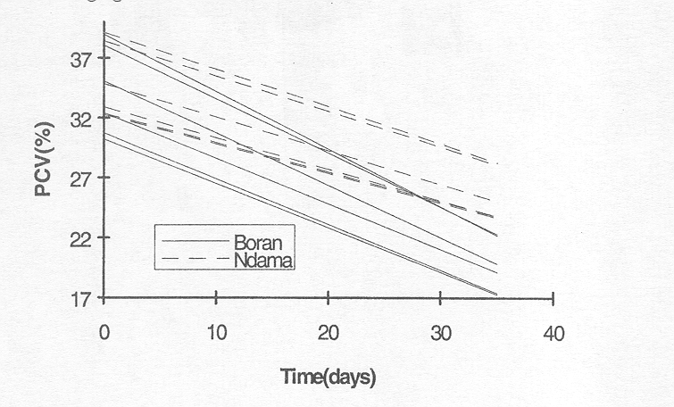
Figure 3.4.2 Change of PCV in time for individual animals based on Model 3. Bold dots and dashes indicate more than one animal with this line.

Compared with the previous analysis this figure demonstrates that PCVs tend to decrease more rapidly the higher the initial PCV. This illustrates the negative covariance between slope and intercept observed in the fitting of the model.