Appendix F

Denominator degrees of freedom

In the first part of this appendix, we will concentrate on the fixed effects model and once we know how denominator degrees of freedom can be determined in that framework we will proceed with the mixed model.

Assume that we want to test a testable hypothesis, i.e., the hypothesis can be stated in terms of an estimable function c^T

H₀ : c^T = 0
H_a : c^T<>0

A typical test statistic is

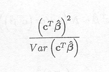
which can also be written as

Note that Var (c^T) is assumed to be known. In the case that this variance is known, the test statistic has a Chi-square distribution with 1 degree of freedom. In practice, however, the variance has to be estimated from the data.

We will restrict to the simpler case of the cell means model. In a fixed effects model, the variance of an estimable function can be easily obtained

An estimate of this variance can be obtained by substitution of  ² with the sampling variance s², which is equal to the error mean square.

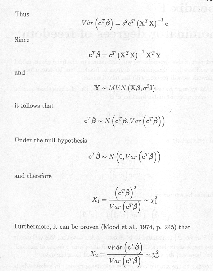
where v corresponds to the degrees of freedom of the mean square error.

As X_l and X₂ are independent from each other (Searle, 1971, p. 190), it follows that

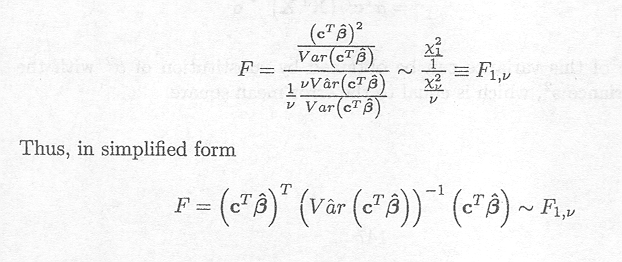
As an example, take the simplest fixed effects model where all observations are independent and, under the null hypothesis, have a common normal distribution with mean µ₀ and variance σ ², i.e., Y₁, Y₂, Y_n ~ N (µ₀, σ²).

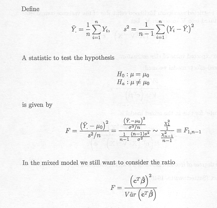
However, due to the more complicated structure of Var (c^T) and Var (c^T) the denominator degrees of freedom in this ratio is more complicated. In fact we mimic for mixed models the methodology that is, under the assumptions of normality, correct in the fixed effects model; as a result we propose an approximate F-distribution for the distribution of

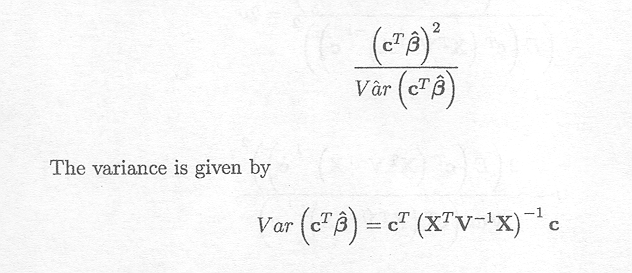
As estimator we use

where the restricted maximum likelihood estimates of the variance components are substituted into V to obtain V. Let

denote the expected value of this estimator.

For the fixed effects model we used

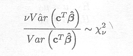
A 'substitute' for this in the mixed model is

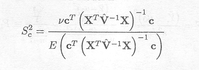
with v the degrees of freedom associated with the estimator .

We now act (Satterthwaite, 1946) as if

By the Chi-square distribution assumption, it follows that

Var (S) =

or equivalently

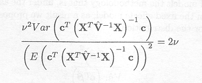
Thus

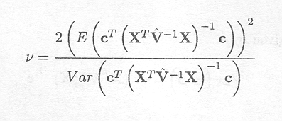
Giesbrecht and Burns (1985) proposed the following approximation, based on a Taylor expansion for the term in the denominator,

An approximation for v is then given by