Contents
1. Introduction
2. General concepts
3. Fitting a straight line
4. Analysing a randomised block design
5. Statistical inference
6. Comparisons between means
7. Simple analysis of discrete data.
8. General statistical models
9. More advanced regression models
10. Models for proportions
11. Models for counts
12. Models for times to an event
13. Multi-level data and mixed models
14. Repeated measures
15. Analysis of field studies
16. Other models
17. Related reading
The Exploration & description guide has described the steps involved in undertaking exploratory methods of analysis in order to obtain first impressions of the patterns that exist in the data and to suggest further statistical analysis. By the time that this next phase is reached clear objectives will have been set to define explicitly the types of statistical analyses required and the models to be fitted.
During the exploratory phase it is not always possible to look at the effects of a number of different sources of variation simultaneously. The different patterns that have emerged now need to be put together and analysed in a way that can reveal the ones of greatest significance. This is where statistical modelling can play an important role.
Not only can one get estimates of the parameters describing the effects of the variables of most interest, adjusted for the influence of other variables, but one can also subscribe measures of precision (in the form of standard errors) to the estimates and test for their statistical significance. Thus, when fitting straight lines (for example, for studying milk offtakes in cattle in Case Study 1) or determining mean values for different groups of data (for example, for breeds of sheep in Case Study 3) one can simultaneously take into account other sources of variation that contribute to the pattern and, by doing so, hopefully reduce the residual variation too.
We cannot cover within this guide every type of statistical model that one might encounter in research. So we shall mainly focus on concepts. Our approach is to demonstrate the general philosophy of statistical modelling, so that by the time the student has tackled a few of the case studies he/she will have a better understanding of the types of approaches to follow when analysing research data. University of Reading Statistical Services Centre have produced a number of Good practice guides on analysis that can be read in conjunction with this teaching guide. A reader who is dealing especially with the analysis of survey data should take particular note of Good practice guide No. 17.
As has already been discussed in the Exploration & description guide, data can be of various types: continuous, discrete, which can be ordinal, nominal or binary, proportional and elapsed time. Furthermore, they can be multi-structural in nature and occur at different layers, for example, at province, district, village or household levels. The statistical methods and the assumptions involved in modelling vary for the different types of data, but the general approaches are the same.
In this guide we shall develop the general ideas and concepts behind statistical model formulation and analysis by using normally distributed, continuous data structured at one layer, and then later show how the techniques can be extended to other types of data at single or multiple layers.
Before moving on one needs to have a good idea, as discussed at the end of the Exploration & description guide, of what needs to be achieved in the modelling phase. A lot of time can be wasted trying out different data analyses without any particular strategy in mind. Thus, it is a good idea to set down the primary analytical objectives, and ways to meet them, prior to starting to fit models. They will include lists of:
Students should not be put off by the occasional formulae that appear in statistical courses. The few that are included in this guide are done so intentionally in order to help with the general understanding of the concepts. Students will also be able to relate the formulae to those that appear in their lecture course notes or text books.
It is helpful to know how statistical models are constructed so that one can understand and critically review analytical descriptions of statistical methods appearing in research reports.
The underlying concept in statistical modelling is that of formulating a model of the form:
data = pattern + residual
The 'data' are the raw data that have been collected, or sometimes data that have been prepared for analysis and derived from the original data. These might, for example, be transformed values (as discussed under Exploration & description) to meet the assumptions (described later) for least squares analysis of variance, or calculated proportions for use in logistic regression.
Data that are used in an analysis may also be mean values derived from the raw data. For example, Case Study 10, that describes the statistical analysis of longitudinal data used to assess the impact of tsetse control on cattle productivity, uses mean values for analysis that have been calculated over selected periods of time.
The 'pattern' is an expression made up of the various variables, data groupings, factors and covariates etc. that feature in the design of the study or have been selected during the exploratory phase to explain different sources of variation in the data.
The 'residual' is the variation that remains and is not contained within the pattern. If the pattern evident amongst a set of data points can be represented fully by the fitted model then the residual term simply represents pure random variation. If not, then some non-random components will remain within the residual term.
The aim of statistical modelling is to put as much of the variation as possible into the pattern, whilst keeping the model as simple as possible. Of course, the success in fitting a statistical model is dictated by the degree to which the data display significant patterns. There is also the danger of making the model too complicated in the sense that the model over-fits the data and mistakenly incorporates some of the residual variation in the pattern itself.
Over-fitting of a model is discussed in Case Study 3 in relation to the fitting of a curve to express the variation among weaning weights of lambs grouped by different ages of ewes. It is also discussed under Models for proportions in relation to the analysis of data that supposedly follow a binomial distribution, yet the value of the residual deviance suggests degrees of 'under dispersion'.
We have already, without realising, come across the simplest form of statistical model when we calculated a mean in the previous Exploration & description guide. Thus, the model
data = mean + residual
can be used to describes how a single sample of observations has a mean (m, say).
Since biological observations naturally vary one from another, for genetic or environmental reasons, each will deviate from the mean by a value e, say, which is the error or residual term that represents the random component for that observation. Algebraically, we can write this as:
yi = m + ei (i =1,..., n)
where yi (i = 1,..., n) are the observations, m the mean and ei (i = 1,..., n) the corresponding residuals, which, for a correctly specified model, represent just random variation. We saw in the
Exploration & description
guide that the sum of squares of ei (which is equivalent to  (yi - m)2 as derived from the above formula), is used in the calculation of a variance.
Methods of statistical modelling are often described under different headings such as linear regression, multiple regression, analysis of variance, analysis of covariance, generalised linear models, logistic regression, log-linear models, hierarchical models, mixed models etc. Whilst there are subtle differences in the mathematical methods used for fitting these different models, the overall concepts in model fitting are nevertheless the same.
Although we cannot ignore these commonly used traditional names, we shall treat the subject more broadly and demonstrate, whatever the particular attributes of a statistical method, that there is a common approach to model formulation, analysis and interpretation. Just as for Study design this may prompt some changes in the teaching/learning of statistical modelling so that the student has a better appreciation of what is involved in the general approach to statistical model building.
Various terms exist in the literature to describe the terms that occur in a statistical model. Thus, the word 'independent variable' is often used to describe a variable (usually a quantity subject to continual increase or decrease) that sits on the right hand side of a regression equation. Sometimes the word 'explanatory variable' or 'predictor' is used instead. The variable on the left hand side is usually referred to as a 'dependent variable' or 'response variable'.
Likewise, in analysis of variance of designed experiments the terms that sit on the right hand side are often described as 'parameters' or 'factors', or some times 'fixed effects'. They are usually in the form of groupings or sets of categories (for example, blocks, treatments, factors or some other form of grouping), but they can also include 'independent' variables, such as used in analysis of regression. These are often called 'covariates'. Indeed, there is a considerable overlap in the definitions used for different 'types' of analysis.
We shall try to stick to the term 'classification variable' or 'factor' to describe a term in a model that is composed of a set or group of categories, and 'independent variable' to describe a 'continuous variable'. We shall try to remember to use the word 'response variable' to describe the variable that is being measured and occurs as 'data' on the left hand side of the equation.
Variables with increasing or decreasing ordinal values can be treated either as factors or continuous or independent variables. An independent variable is represented by a single parameter, whereas a factor or classification variable is represented by several parameters that describe the different levels or categories.
Note that a variable with two levels (0, 1 or 1, 2) can be fitted either as a factor (see variable LOCATION in Case Study 1 that fits a regression model to milk offtake of cows) or as an 'independent variable'. Although taking on nominal values the variable LOCATION can also be treated as an independent variable (the 'direction' depending on which way the levels are coded).
When fitted as a factor the parameter estimate is interpreted as a difference in mean values; when fitted as an independent variable the estimate represents the slope of the line joining the two means, which are one unit apart [tan Ø = (![]() 2 -
2 - ![]() 1)/ (2 - 1)]. By diagrammatically sketching in the form of an x-y plot the way that these two methods determine the two estimates, it is possible to appreciate that the results are indeed the same (Fig.1).
1)/ (2 - 1)]. By diagrammatically sketching in the form of an x-y plot the way that these two methods determine the two estimates, it is possible to appreciate that the results are indeed the same (Fig.1).
Fig. 1 Illustration of alternative methods for calculation of the difference between two means when parameter fitted either as factor or as an independent variable.
As we shall see later, all models, however simple, can be considered within the framework of general statistical models that can contain mixtures of independent variables and classification variables or factors. The term 'fixed effect' is an all-embracing term for this mixture of variables, generally used within the mixed model framework to distinguish them from random effects. This will be described later under Multi-level data and mixed models.
Most statistical analyses, even regression analysis, use some form of analysis of variance (or in certain cases analysis of deviance) and these provide the basis for presenting a general approach to statistical modelling. An understanding of how simple models are constructed and analysed can give the student a general understanding of the principles of statistical model formulation and analysis, so that he/she can appreciate what is happening when a more advanced model is being fitted.
Next we describe in some detail the formulation and analysis of models for the fitting of a straight line and for the analysis of data arising from a randomised block design.
Small data sets can be extracted from those associated with Case Study 1 and Case Study 8 to which the student can apply these simple calculations by hand. By using GenStat, Instat or another statistical package the student can then verify that his/her solution matches those of the program. It is also an informative way of appreciating how the computer output is presented by a software package and what each item means.
Commonly known as simple linear regression, the approach involves the fitting of an equation to a straight line that best represents the pattern in variation between two variables y and x. The response variable y is usually assumed to be continuous, i.e. it can take on any reasonable value within a given range. The independent variable x can be continuous or ordinal. In terms of the idea that
data = pattern + residual
we can describe the expression in the form of an equation of the form:
y = a + bx
where a is the parameter that describes the point where the line intercepts the y-axis, and b is the slope or the gradient of the line. Since there will be a random scatter in the data values, we need to add an extra term to the equation to represent the deviation of an individual point from the straight line. Our complete model for the data is therefore:
y = a + bx + e
where e represents the deviation of an individual point from the line, i.e. the residual (or error) term. We often attach a suffix i to the y, x and e letters to signify a particular data item i. Thus, assuming there to be n (x,y) observations, we can write the above equation
yi = a + bxi + ei (i = 1, ...., n ) ---------------(1)
The sum of the eis is zero. Fig. 2 shows an example, taken from Case Study 3 of a straight line superimposed on a scatter of the points. The vertical distance from a point to the position on the line represents the size of the residual ei for the particular point yi. The method used for finding the line that best fits the data is known as the 'method of general least squares'.
The method of least squares is the one that is usually applied in the derivation of an analysis of variance to describe the pattern presented by different forms of a statistical model (e.g. regression analysis, designed experiments etc.).
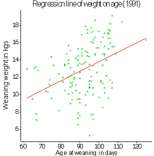
Fig.2. Illustration of a straight line fitted by the method of general least squares to observations representing weaning weight of lambs and their age at weaning. (Data taken from Case Study 3).
We compare by analysis of variance the amount of the variation in the yis that contributes to the positioning of the straight line through the points to that that is left over. Analysis of variance is a tool applied across a wide range of different statistical analyses. It describes the amount of variation that can be explained by the pattern described by the model, and compares the size of this variation to the remaining or residual variation that does not contribute to this pattern.
An analysis of variance table comprises five columns: source of variation, degrees of freedom (d.f.), sum of squares (S.S.), mean square (M.S.), which is equivalent to the sum of squares divided by the degrees of freedom, and variance ratio (V.R.), which divides a mean square associated with a pattern (in this case a straight line) by the residual mean square. The residual or error mean square is an estimate of the residual or error variance.
The total mean square (not usually presented in a computed analysis of variance table) represents the variation (variance) in the data before any pattern (in addition to that represented by the overall mean) is investigated.
When fitting a straight line the analysis of variance table looks like:
Source of variation |
d.f. |
S.S. |
M.S. |
V.R. |
Slope of line |
1 |
|||
Residual (error) |
n-2 |
|||
Total |
n-1 |
To understand how the analysis of variance handles the calculation of the intercept (a) and the slope or gradient (b) of the line we can add up equation (1) for each of the xis and yis and then calculate the averages  and
and  .
.
Since the sum of the eis is zero we have = a + b.
Switching the equation around we have a = - b
Substituting for a in equation (1) we get
yi = - b
+ bxi + ei
= + b (xi- ) + ei
Thus, in fitting the straight line we need to calculate the mean values for and and estimate the slope b.
As already stated, the total mean square in the analysis of variance table represents the variance of the yis before any pattern is fitted. The estimate is used for calculating this variance, and so the degrees of freedom are reduced from n to n-1. If we stop here then we have a horizontal line through the mean of the points parallel to the x-axis. All we need to do now is to rotate the line so that it best accounts for the pattern in the data points. In doing so, we need one more parameter, namely the slope b to describe the direction of the line.
For simple examples, such as fitting a straight line, it often helps if students can understand how the calculations are done. Having gone through this process they are then in a better position to appreciate the types of calculations that will be applied in more complicated cases.
The formulae for regression analysis are well documented in text books but for completeness they are shown here. The sum of squares for the yis is calculated as
![]() yi2 - (yi)2/n. This is precisely the formula used for the numerator in the calculation of a variance (Exploration & description). It helps, in what follows, to give this expression a shorthand notation Syy.
yi2 - (yi)2/n. This is precisely the formula used for the numerator in the calculation of a variance (Exploration & description). It helps, in what follows, to give this expression a shorthand notation Syy.
Using the xis we can similarly calculate Sxx = xi2 - (xi)2/n, the sum of squares for the xis. Sxy is calculated as xiyi - (xiyi)/n, i.e. the sum of cross products.
Using these expressions it can be shown that the sum of squares column in the analysis of variance table is composed of:
Source of variation |
d.f. |
S.S. |
M.S. |
Slope |
1 |
(Sxy)2/Sxx |
|
Residual |
n-2 |
Syy - (Sxy)2/Sxx |
|
Total |
n-1 |
Syy |
Each line in the M.S. column is then calculated as (S.S. / d.f.) using the corresponding S.S. and d.f. values. If the mean square for the slope is greater than the residual mean square then it can be deduced that the residual variance has been reduced to a value below that for the total M.S. The larger the variance ratio the greater is the reduction in the residual variance, and so the clearer is the pattern.
Later under Statistical inference we shall discuss methods for attaching levels of probability to the likelihood that a pattern is real, but, for the time being, the student should try to make his/her own judgment based on the size of the variance ratio alone as to the likelihood of the pattern being real or not.
It is a good idea to impress on the student the importance of parameter estimation relative to statistical significance testing. The student also needs to be informed that statistical significance does not necessarily imply biological significance.
The following expressions can also be calculated:
 (residual M.S. / Sxx)
[(Sxy)2/(Sxx x Syy)]
(residual M.S. / Sxx)
[(Sxy)2/(Sxx x Syy)]
The standard error (s.e.) measures the precision with which the estimate of the slope b is determined. We can use this standard error for determining a confidence interval for b in the same way as shown in
Exploration & description for a sample mean
![]() .
.
The correlation coefficient (usually written r or p) provides a measure of how well the two variables x and y are associated. The coefficient can lie between 0 (indicating no association) and 1 (perfect association, i.e. all points lie on a straight line). The correlation coefficient is usually used to define the association between two variables when neither takes on the role of the response variable. In other words both variables can be considered as independent variables in the analysis.
A student could usefully apply these calculations by hand to a simple data set and then run the same analysis with GenStat, Instat or other statistical package to see how the results compare.
So far we have considered the fitting of an independent x-variable in a simple linear regression model assuming that it is a variable that covers a continuous range. The x-values may be continuous, i.e. take on any value within a given range, or they may be ordinal, perhaps representing a range of increasing factor levels.
Thus, Case Study 9 illustrates how a regression curve is fitted to see how pollen germination of the perennial leguminous Sesbania sesban tree is related to sucrose concentration. The aim was to predict pollen germination at any point over the range of sucrose concentrations used in the experiment.
Sucrose concentration, however, can also be analysed as a factor with each level representing a different sucrose concentration level. Thus, the aim of the data analysis in Case Study 9 was first to examine the effect of each level of sucrose concentration on pollen germination, and then to see how the variation among concentrations could be represented by a curvilinear relationship.
A randomised block experiment yields parameter estimates that take on a different form from those for independent, continuous variables. They are represented and analysed differently. For example, the blocks in a crop experiment will usually be numbered, e.g. 1, 2 and 3, but the numbering is not necessarily related to potential yield. Likewise, treatments will often be distinct entities, e.g. vaccine treatment, positive control, negative control, and again there is no particular nominal order. Thus, the formulation of the statistical model for a randomised block experiment is a little different from that for a linear regression analysis. Nevertheless, the concept is the same in that both methods are fitting the same model:
data = pattern + residual
Thus, we are again interested in seeing how much of the total variation in the data can be ascribed to a pattern associated with the different treatment levels. For the moment we assume that the response variable is continuous. We shall consider later situations where the variable is discrete (e.g. diseased or not).
Let us assume that we are dealing with an experiment on Napier grass with treatments assigned at random to plots within different blocks or replicates. Case Study 5 describes such an experiment with several different accessions planted in three replicates.
The yield of Napier grass achieved within a certain plot will to some extent be a consequence, not only of the treatment that is applied to the plot, but also of the fact that the plot lies within a particular block. The block may cover a horizontal area where the ground has a particular slope or an area that is shaded by trees, and so all plots in the block will tend to share some of the variation associated with the block.
Nevertheless, all the plots within the block will not be expected to have the same yield; otherwise there will be no random residual variation. It is this residual variation that will remain after the pattern that describes the treatment and block effects has been determined.
Just as we described algebraically the fitting of a straight line, so we can do likewise for the estimation of mean values for different treatments. By understanding how the model is formulated in the simple case of a randomised block the student should be better able to grasp the general concepts of a statistical model and how it is put together.
Suppose we use the letter r (not b) to refer to block (replicate), so as not confuse with the letter b used earlier for slope, and use t to refer to treatment. We shall assume that that the randomised block experiment includes four treatments and three blocks.
Let us give a suffix to each r and t to define the particular block (r1, r2, r3) and treatment (t1, t2, t3, t4) to which a plot belongs. We can now describe the yield of Napier grass from the plot from block i (i = 1, 2, or 3) and treatment j (j = 1, 2, 3, or 4) with two suffices i and j side by side. Thus, for the first plot we can write
y11 = r1 + t1 + e11
where y11 represents the yield for the plot in block 1 that is given treatment 1, and e11 represents the component that cannot be ascribed to the pattern expressed by r1 and t1. Similarly, for treatment 4 in block 2 we can write
y24 = r2 + t4 + e24
Usually, r and t are defined as deviations from the overall mean, which is usually written using the Greek letter µ. Thus, in practice the above two equations are expressed as:
y11 = µ + r1 + t1 + e11
y24 = µ + r2 + t4 + e24
There are 12 (3 x 4) equations which can similarly be written. We can define a single algebraic expression that allows them to be written together as:
yij = µ + ri + tj + eij (i = 1, 2 or 3; j = 1, 2, 3 or 4)
This is the algebraic expression for the expression
data (y) = pattern (µ + r + t) + residual (e)
Case Study 8 describes a form of a randomised block experiment used for feeding goats. The 'blocks' here, however, are somewhat different from those used in agronomy and represent different batches of goats fed over time. This case study also gives an example of unequal replication of treatments (diets) within batches.
An example of a completely randomised design is given in Case Study 13 which also compares different feeding regimes in goats. The statistical model for this design includes only a 'treatment' term.
The layout of a randomised block experiment might look like:
Block 1 (r1) |
t1 |
t3 |
t4 |
t2 |
Block 2 (r2) |
t2 |
t3 |
t1 |
t4 |
Block 3 (r3) |
t4 |
t1 |
t2 |
t3 |
As has already been mentioned, the purpose of analysis of variance is to separate and quantify sources of variation associated with certain patterns. There are two sources of variation in this example - block and treatment. The analysis of variance may thus look like:
Source of variation |
d.f. |
S.S. |
M.S. |
V.R. |
Blocks |
2 |
|||
Treatments |
3 |
|||
Residual |
6 |
|||
Total |
11 |
Note that the numbers of degrees of freedom for blocks are 2 = (3-1) and those for treatments 3= (4-1).
To understand how the degrees of freedom are calculated consider the degrees of freedom for blocks. As in linear regression the overall mean (µ) is estimated by the mean
![]() averaged over the 12 observations yij. The three block means are thus represented by the expressions (
averaged over the 12 observations yij. The three block means are thus represented by the expressions (![]() + r1), (
+ r1), (![]() + r2) and (
+ r2) and (![]() + r3), respectively. The average of these three means must equal
+ r3), respectively. The average of these three means must equal
![]() . We can therefore write:
. We can therefore write:
[(![]() +r1) + (
+r1) + (![]() + r2) + (
+ r2) + (![]() + r3)]/3 =
+ r3)]/3 = ![]()
It follows that r1 + r2 + r3 = 0
Thus, once values for r1 and r2 have been derived within the analysis it is a simple matter to calculate r3 by subtraction. In other words, once the overall mean is known, we only need to calculate the parameters for two of the three blocks; the third depends on the first two. The same pattern applies for treatments - once t1, t2 and t3 have been derived, t4 can be obtained by subtraction. Thus, blocks and treatments have 2 and 3 degrees of freedom, respectively.
Thus, the ris and tjs are constrained by the relationships r1 + r2 + r3 = 0 and t1 + t2 + t3 + t4 = 0, respectively, so that r3 = -(r1 + r2) and t4 = -(t1 + t2 + t3). Statistical computer programs often use an alternative constraint and set the first of the parameters (in this case r1 and t1) to 0. Thus, only r2 and r3 and t2, t3 and t4 are estimated. This also means that the parameter µ takes on a different meaning. It becomes the estimate of the first treatment mean in the first block.
By showing how the analysis of variance table is calculated we continue to illustrate the general concept of distinguishing between 'pattern' and 'residual' or 'error'.
For a simple randomised block we first sum the yijs to calculate block totals R1, R2 and R3, treatment totals T1, T2, T3 and T4 and a grand total G.
The general formula for the sums of squares for blocks in a randomised block with r blocks and t treatments, and equal replication of treatments within blocks,
= (R12 + .....+ Rr2) / t - G2/rt
Each Ri2 in the above equation is divided by the number of observations that contribute to the total, in this case t. Thus, in our particular example there are four observations in each block, so
block sum of squares = (R12 +R22 + R32) / 4 - G2/12
Similarly, there are three observations for each treatment, so
treatment sum of squares = (T12 + T22 + T32 + T42)/ 3 - G2/12
The total sum of squares is calculated as for fitting a straight line.
The residual sum of squares is calculated by subtracting the block and treatment sum of squares from the total sum of squares.
Mean squares are then calculated by dividing each of the sums of squares by their corresponding degrees of freedom, and the variance ratios for treatments and blocks by dividing their respective mean squares by the residual mean square. Again the larger the variance ratio the greater is the likelihood that the source of variation contributes significantly to the overall pattern.
The different treatments can either be presented as parameter estimates (t2, t3, t4, say), which represent the deviations of treatments 2, 3 and 4 from treatment 1, or as least squares mean estimates which incorporate the estimate of the value for µ.
In the simple case of a balanced randomised block design the least square means are the same as the arithmetic means of the observations recorded for each treatment. When there is imbalance in the study design, however, the statistical analysis makes adjustments for this lack of balance and presents results that simulate the situation that would have arisen had there been no imbalance.
When presented as parameter estimates the first treatment (t1) is defined as the reference level (value 0) and other estimates as deviations from t1.
Now suppose that there is a factorial arrangement of the treatments with factor A at two levels and factor B also at two levels. We can derive a similar statistical model for A and B, also their interaction. By using letters a and b to represent the two factors we can write the model
yijk = µ + ri + aj + bk + (ab)jk + eijk
The writing of ab within parentheses is a commonly used practice to describe the interaction between two factors. Note that we now need to use three rather than two subscripts to describe the model. The analysis of variance now looks like:
Source of variation |
d.f. |
S.S. |
M.S. |
V.R. |
Block |
2 |
|||
A |
1 |
|||
B |
1 |
|||
A x B |
1 |
|||
Residual |
6 |
|||
Total |
11 |
Note that the degrees of freedom for A, B and the interaction term A x B sum to three, the same number shown earlier when the four treatments were presented without a factorial structure.
Calculation of the individual sums of squares for A and B follows a similar form to that for treatments, namely, squaring each total and dividing by the number of observations that contributes to the total, in this case six. The interaction sum of squares can be calculated by subtracting the sum of the sum of squares for A and B from the total treatment sum of squares calculated previously.
If the mean square for the interaction is found not to be significant then we can deduce that the effect of each level of factor A on the response variable is the same irrespective of the level of B (see, for example, Case Study 10, where the interaction between tsetse control (A) and method of application of insecticide (B) was found to be non-significant).
If the interaction is significant then we can deduce that factor A has a different effect on the response variable for the different levels of B. In such circumstance it becomes less meaningful to consider the overall effects of each factor irrespective of the influence of the other. It is more important to decide which means to present for which factor level and which standard errors to present with them.
So far, when commenting on the general size of the variance ratio (V.R.) in the analysis of variance table, we have simply noted that the greater its value the more significant it is. Obviously, if the variance ratio is less than one then there can be no contribution to the overall pattern and the term can be omitted from the model. But how large does the variance ratio need to be for it to be statistically significant?
Statistical theory states that, when the data are independent and can be assumed to be normally distributed from populations with a common variance, the variance ratio follows what is known as an F-distribution.
The F-value has two separate degrees of freedom, the first corresponding to the number of degrees of freedom associated with the numerator, the line in the analysis of variance table that represents the particular component of the pattern, and the second associated with the denominator, the residual term. In the case of the randomised block example with three blocks and four treatments, there are six degrees of freedom for the residual term. Thus, the degrees of freedom for F for the treatment term in the analysis of variance are 3 and 6, respectively, and the F-value is written as F3,6.
The important point to understand is that, when statistical inference is applied in the form of F-tests to interpret the results of an analysis of variance, the assumption is that the eijs are independent, normally distributed and add up to zero.
Tables are available that give the values that F needs to exceed to achieve statistical significance at the 95, 99 and 99.9% levels of probability, respectively. For F3,6 these values are 4.76, 6.60 and 9.78, respectively. Thus, if the value of the variance ratio for treatments in the analysis of variance table is greater than 4.76 we say that the difference among treatments is significantly different (P<0.05). If the variation ratio is greater than 6.60, then the statistical significance level is P<0.01, and, if greater than 9.78, then P<0.001.
When the numerator degrees of freedom is 1, it can be shown that F1,6 = t62, namely the square of the t-value for comparing two means. This provides an analogy between an analysis of variance and a t-test (see Comparison between means). Thus, the process for calculating an unpaired t-test to compare two means corresponds precisely to that for a one-way analysis of variance for a completely randomised design with a factor at two levels, though on a different scale. Similarly, a paired t-test corresponds to an F-test in an analysis of variance for a randomised block design with two treatments and two blocks. Thus, behind the application of any t -test there also lies a statistical model.
Researchers should not get carried away with a need to obtain statistical significance differences. Further reasons for doing so are discussed in the Reporting guide. This is not because the ability to attach a significance level to a result is unimportant, but rather that it is only a tool for use towards meeting the objectives. Of more importance is the estimation of mean values and the attachment of standard errors to them in order to measure the precision to which the mean values have been determined.
Having done an analysis of variance and found a statistically significant F-value, the researcher may wish to know how the means obtained for each level of the classification variable differ one from one another.
Multiple range tests became popular some years ago but are often misused. They are suitable only in cases where there are a large number of levels to compare for a classification variable and when the levels are nominal and there is no intrinsic structure among them. Thus, such tests may be appropriate in large variety trials where there is no preconceived idea of how each variety is likely to perform. Such a test could have been applied in Case Study 5, for example in which different accessions of several Napier grass accessions were grown.
In a trial where different levels of a treatment, say a fertiliser, are being applied, increasing quantities are likely to feature in the treatments being given. It is more likely that the researcher is looking for an ideal level of fertiliser and this will have been an objective set down for the study. Multiple range tests are not appropriate in this case. The researcher is better off applying, in an intelligent way, simple t-tests between pairs of means.
The formula for the t-test, when means have the same number of observations, is
t = (![]() 1 -
1 - ![]() 2) /
2) / ![]() where
where
s2 is the residual variance and n is the number of observations per mean.
When the numbers of observations that contribute to each mean are different, the formula becomes:
t = (
The value for the residual mean square in the analysis of variance table can be used as an estimate for s2.
Mean comparisons can also be done within the analysis of variance framework using what are sometimes known as 'contrasts'. Suppose, for example, it is required to compare the mean of a number of treatments with the control. We have seen how it is possible to work out the standard error for this comparison by substituting values for n1 (summed over treatments) and n2 (for the control) in the above formula and then to apply a t-test. But the same comparison can likewise be applied within the framework of the analysis of variance by describing the same relationship in the form of a contrast. Most statistical programs provide this facility. The contrast is evaluated using a F-test and provides the same result but on a different scale (F1,n = tn2).
So far we have been dealing with the situation when the response variable y is continuous and the error distribution is normal. Now we turn our attention to a situation where the response variable is discrete in nature. There are general methods for the analysis of discrete data, for example 0 or 1 responses, similar to those for continuous data. These methods extend the range of models that we have been considering so far to a broader family of 'generalised linear models' (see Models for proportions)
There are many situations, however, where discrete data can be summarised simply in two-way tables (known as contingency tables) and analysed using a X 2 test. Often, such an analysis may be all that is required (see, for example, Case Study 11 that summarises ownership patterns of livestock by gender of the head of the homestead in a livestock breed survey in Swaziland).
To show how a X 2 value is calculated, suppose that r1 from n1 cattle exposed to trypanosomosis die during a year when no preventive treatment is applied, and that r2 from n2 cattle similarly die in the following year when a preventive treatment is taken. We can put the values into a 2 x 2 table and apply a X 2 test.
Without prophylaxis |
With prophylaxis |
Total | |
Died |
r1 |
r2 |
r1 + r2 |
Survived |
n1 - r1 |
n2 - r2 |
n1 + n2 - r1 - r2 |
Total |
n1 |
n2 |
n1 + n2 |
The method is described in text books and so little more needs to be added, except that we do need to know how many degrees of freedom to use before looking up a table of X 2 values. To show how we can find out, assume that the five values in the row and column totals in the above table are given. Then, as soon as we put a value into one cell of the table, say r1, the values in the other three cells can be derived immediately. In other words we can conclude that only one degree of freedom is needed.
Similarly, as soon as we have inserted values for two cells in a 3x2 table the values in the remaining four cells can be derived. Thus, the number of degrees of freedom is 2 (or (3-1) x (2-1)).
A useful definition to introduce here is that of the 'odds ratio'. It is calculated as
[r1/(n1-r1)] / [r2/(n2-r2)]
and represents the odds of an animal dieing in the first year when no preventive treatment is applied, compared with the odds of an animal dieing in the following year when preventive treatment is applied. An 'odds' on its own is the number of animals in either of the columns that died expressed as a proportion of those that did not. This term will be discussed later when more general models of proportional data are considered (Models for proportions).
We sometimes need to be careful in interpreting the results of X 2 tests when applied to contingency tables. When we compare the proportions that die with and without treatment we are considering the relationship
data = pattern + residual
The data considered above are the numbers dieing or not dieing and the pattern a comparison between those without treatment in the first year and those with treatment in the second year. When considering the effect of treatment in this case, however, we are ignoring the fact that the comparison takes place across different years. In other words we are not able to distinguish between treatment and year.
When applying X 2 tests in two-way tables it is important to remember that the pattern has only one component, namely the comparison being made, and that any other factor that may exist in the background and may be of significance is being ignored. If other factors are likely to be important, then one should ensure that the design of the study is suitable to allow for such partial confounding and to enable a more general statistical model to be fitted (see Models for proportions).
Sample sizes for discrete data generally need to be larger than for their continuous counterparts in order to achieve the same level of statistical significance. Sometimes data sets are too small to study more than the simplest types of pattern.
Simple illustrations are given above on how statistical models are formulated and evaluated. The parameters on the right hand side of an equation can be of two types: independent variable (when fitting a straight line) or a grouping or classification variable (such as a treatment or block in an analysis of a randomised block design). Both types of variables, however, result in similar forms of analysis of variance. Although the algebraic expressions for these models may look a little different they are both fitting the relationship
data = pattern + residual
and in each case the method of analysis is by the general method of least squares.
Indeed, it is possible for independent and classification variables to be put together in the same model. Thus, a generalised expression for a statistical model can look like:
yijk = µ + ri + sj + tk + (rs)ij + (st)jk +b1xijk + b2zijk + eijk
where i = 1, ...., ni, j = 1, ...., nj, k = 1, ...., nk. When the y-variable is continuous the method of analysis will be by the method of least squares. The parameters ri, sj and tk are assumed to represent classification variables and xijk and zijk independent variables. The model also includes, for illustration purposes, two interaction terms.
The analysis of such statistical models results in an analysis of variance with each term (except eijk) in the equation contributing to the overall pattern. As has been shown, calculations can be done by hand for a randomised block design or simple linear regression. However, in an unbalanced design calculations by hand become more difficult and are better done by computer.
Data can often be unbalanced, for instance when classification variables, such as those in the above model, are not equally replicated at each level. This often results in partial confounding between the different terms in the model. It is then important to decide on the order in which terms should be included in the analysis.
As each term is added to the analysis of variance table the calculated sum of squares that is calculated is the additional amount attributable to the introduction of the new term with the proceeding terms in the model already fitted. The first term to be included in the analysis ignores any contributions to the sum of squares from the remaining terms. Thus the order matters.
A good illustration of this is shown in Case Study 3. When lamb genotype is included first in a model fitted to weaning weight the sum of squares equals 570.427 kg2, but when the contributions of the other variables are taken into account first, and genotype is added last, the sums of squares for genotype reduces to 75.857 kg2. This is the value that we need to know as it represents the independent contribution of the variation among the genotypes, and discounts the variation (570.427 - 75.857 = 494.570 kg2) that overlaps and cannot be distinguished from the variations associated with the other variables.
When data are balanced (i.e. orthogonal) such as in the 3x4 randomised block discussed earlier, it does not matter in which order the sums of squares are calculated, for the sums of squares for block and treatment are independent of each other, i.e. there is no overlap.
Variables, such as age, sex, pre-trial milk yield that are not involved in the study design are often recorded with the possibility of using them as covariates to explain some of the variation in the response variable. They can be incorporated in the model as independent variables alongside the classification variables. Sometimes such an analysis of variance, when applied to a designed experiment, is referred to as an 'analysis of covariance' and the independent variable as a 'covariate'. Case Study 8 uses an analysis of covariance for milk yields of goats with pre-treatment milk yield as a covariate.
Parameters describing estimates of factors or classification variables and parameters giving estimates of regression coefficients for independent variables will usually be listed together in a computer output. Unlike the sums of squares in the analysis of variance, however, these parameter estimates are calculated from the complete model, and are thus adjusted for the presence of the other variables. In other words, they are derived assuming that the variable that they represent is the one added last to the analysis of variance table.
The parameter estimate for the first level of a classification variable is usually omitted by the computer program (see discussion on parameter constraints in Analysing a randomised block design), and so the other parameter estimates represent deviations from the first level. This first level is often referred to as the baseline or reference level. The parameter estimate for the overall constant µ is not then the overall mean. Instead it represents the 'average 'value when all classification variables take on their first level and independent variables have the value zero.
Adjusted (or corrected) means (often referred to as least squares means) can also be calculated instead of parameter estimates. It is important to note that these least squares means provide estimates of mean values assuming complete balance in the design. Occasionally, this can result in distorted values.
The data set used by Case Study 2 provides a suitable illustration of how such distortion can happen. The lactation number (1 or >=2) for each cow was recorded in the data set. The analysis described excluded cows in their first lactation. However, should all the cows have been retained and lactation number been included as a term in the model, then the calculated least squares milk offtake means would represent the situation when there is an equal number of cows in their first and in all subsequent lactations in the herds. Such a situation, of course, is most unlikely to occur in practice. Manual adjustments can usually be made to the means to ensure that the weighted average of the least squares means equals the overall average in the study.
Sometimes missing values may occur in a designed experiment. Two options are possible.
Firstly, when the data are orthogonal, i.e. there is no confounding between variables, for example, blocks and treatments in a randomised block design with equal replication of treatments across blocks, the data can be analysed with missing value codes (e.g. -999) put into the positions where the data are absent. A general statistical computer program will be able to use the remaining data to estimate these missing values and proceed with the analysis of variance as normal, preserving the orthogonality and adjusting the degrees of freedom to account for the numbers of values that have been estimated.
Alternatively, the analysis can proceed without estimating missing values. In this case the orthogonality is lost and the data used for the analysis become unbalanced.
Interpretation of statistical output from balanced designs is usually more straightforward than from unbalanced designs, but there is a practical limit on the number of missing values that can reasonably be estimated to preserve the balanced nature of the design.
Typically, one, two or three missing values can be readily estimated, but as the number increases beyond that the researcher will need to make a decision between the two alternative methods. The choice of approach relates to the number of values that are missing in proportion to the total number of experimental units.
An ability to write and understand a statistical model is fundamental to ensuring that the objectives of data analysis are successfully achieved. As will be seen later it is also an important way of ensuring that the multiple-layer structures in certain data sets are recognised and taken into account. Some of the case studies give algebraic expressions for the models fitted, others not. It will be instructive for the student to investigate the models given (e.g. Case Study 1, Case Study 8 and Case Study 10) and to try and formulate models where they are not (e.g. Case Study 3, Case Study 9 and Case Study 13).
A clear understanding of the concept of statistical model formulation helps to ensure that other aspects of data analysis fall more easily into place.
Generally, simple statistical models are to be preferred to more complex models, especially when there is considerable imbalance within the structure of the data. The more variables that there are in a model the more difficult it can become to interpret the different parameters, especially when there is partial confounding among some of them.
Several types of ancillary data are often collected in surveys or observational studies in an attempt to remove some of the background variation. Only the variables that are important from a biological point of view or have significant contributions to the overall variations should be included in the final model.
Simple linear regression can easily be extended to contain more variables (see, for example, Case Study 6). Instead of there being just one independent variable xi, there may be many: x1i, x2i, x3i.... The model becomes:
yi = a + b1x1i + b2x2i + b3 x3i + ......... + ei
The combination of the independent variables defines the pattern. The method is often described as multiple linear regression, and is a particular example of the more general statistical model discussed in General statistical models. It may be that not all variables contribute separately and significantly to the pattern. In other words, there may be correlations among the independent variables that result in most of the variation in the yis being accounted for by a subset of the xis. It is possible to fit each xi one at a time and examine the size of the additional sum of squares after fitting other variables.
The analysis of variance table will look like:
Source of variation |
d.f. |
S.S. |
M.S. |
x1 |
1 |
||
x2 / x1 |
1 |
||
x3 / x1, x2 |
1 |
||
x4 / x1, x2, x3 |
1 |
||
Residual |
n-5 |
||
Total |
n-1 |
The expression x2 / x1 stands for the variation in the response variable y due to fitting a regression line to the independent variable x2 given that a line has already been fitted to x1. In other words, the expression explains the variation in y associated with x2 having already accounted for any association (correlation) with x1. Correlations will generally occur among the independent variables. The correlation between a response variable and an independent variable in an equation with several variables is referred to as a 'partial correlation'. When a partial correlation coefficient is small the independent contribution of the associated independent variable to the pattern will also be small.
There are different ways of determine the importance of each variable:
Whichever method is chosen it will also be important to use prior biological knowledge, as discussed above, to decide on which associations are sensible or practical. It may sometimes be necessary to include certain variables regardless of the size of their contributions to the sum of squares.
A multiple regression equation can alternatively be formulated using successive powers of a single variable, to provide what is sometimes referred to as a polynomial curve. This looks like a multiple linear regression equation except that one variable and its squared, cubic values etc are used instead of separate continuous variables. The statistical model becomes:
yi = a + b1xi + b2 xi2+ b3 xi3+ ........+ ei
and the analysis of variance table:
Source of variation |
d.f. |
S.S. |
M.S. |
Linear |
1 |
||
Quadratic |
1 |
||
Cubic |
1 |
||
Residual |
n-4 |
||
Total |
n-1 |
where the 'linear', 'quadratic' and 'cubic' expressions represent the contributions of x, x2 and x3 in turn. The equation can contain further powers of x, though in practice the cubic term is likely to be the highest power that needs to be considered. As soon as a mean square fails to significantly exceed the value of the residual mean square, the fitting of the polynomial equation can cease.
Two case studies illustrate the use of this method of curve fitting. Case Study 3 uses the method to deduce that the effect of the age of a dam on its lamb's weaning weight can be modelled by a quadratic relationship. Case Study 9 does likewise by showing that the relationship between pollen germination of Sesbania sesban and sucrose concentration can also be fitted by a quadratic curve.
The general least squares model described in General statistical models for the analysis of continuous response variables with a normally distributed residual term can be considered as one member of a more general family of generalised linear models. The underlying error distributions for other models in this family, however, can be based on distributions other than normal.
Linear logistic regression is the name given to the method used to analyse data that are either proportions y = r/n, where r is the number of successful outcomes from n observations, or binary (0, 1) values, where 1 indicates a 'successful' outcome and 0 not. Such data tend to belong to a binomial, and sometimes a Poisson distribution, and therefore the analytical treatment is a little different.
As before the aim is to analyse the relationship
data = pattern + residual
but, instead of analysing y, as for a continuous variable, we analyse logit (y) which is the function loge [y /(1-y)] where y = r/n. This is indeed the logarithm of the odds [r/(n-r)] defined earlier in Simple analysis of discrete data leading to consideration again of the odds ratio.
Thus, suppose that we have two classification variables si, i = 1 ... ni and tj, j = 1, ...nj. The data that we use for the analysis are the values rij and nij contained within the individual cells of the 2-way ni x nj table of proportions (r/n) classified by si and tj.
This model falls into the category of a generalised linear model, but rather than fitting the linear model directly by general least squares and assuming a normal distribution, the data are first transformed through what is known as a 'link function' before a linear model can be fitted with the specified error distribution. The binomial distribution is usually used for proportional data and the logit transformation used for the link function. Instead of resulting in an analysis of variance table the analysis results in an 'analysis of deviance' table.
Source of variation |
d.f. |
Deviance |
Mean deviance |
Deviance ratio |
s |
ni - 1 |
|||
t |
nj - 1 |
|||
Residual |
ninj - ni - nj + 1 |
|||
Total |
ninj - 1 |
Here the total degrees of freedom are ninj - 1 since we are analysing an ni x nj table of proportions. The deviance column is analogous to the sums of squares column in an analysis of variance. The mean deviance is the deviance divided by the corresponding degrees of freedom and the deviance ratio is the mean deviance divided by the residual mean deviance.
The residual deviance for a model that fits the data well, and ensures that only random binomial variation is contained within the residual term, should approximate to its degrees of freedom. In other words the residual mean deviance should theoretically be close to 1. When this is so, the value for each deviance, which represents, as for the sum of squares in an analysis of variance, the change in deviance due to the inclusion of the current term in the model, follows a X 2 distribution. Its statistical significance can be determined by looking up corresponding significance levels in a X 2 table.
Often, however, especially in surveys or observational studies, the residual mean deviance will be greater than 1. This will be due to extra 'noise' within the data that cause them to be more variable than if they had simply been associated with simple binomial sampling (such as tossing a coin). When this happens the data are said to be 'over dispersed'. In such cases the ratio of the particular mean deviance with the residual mean square needs to be used instead. This ratio approximates to an F-distribution and is used in the same way as in an analysis of variance, with mean deviances for each term in the model compared with the residual mean deviance.
Sometimes the residual mean deviance falls below 1. The model then suggests that the data are 'under dispersed'. The chances are that more variables are being included in the equation than are justified, and the researcher should re-examine the model to decide whether or not any of the variables should be dropped.
A useful rule for the maximum number of parameters p (that is including every single individual classification parameter level) to be used in a model before problems of over-fitting can occur is p < r / 10, where r is the total number of 'successes' in the data set.
An illustration of the use of logistic regression is given in the appendix to Case Study 14.
The logistic regression method can also be used to fit models to binomial (0,1) data. Thus, if N is the total number of observations, the analysis of deviance would look like:
Source of variation |
d.f. |
Deviance |
Mean deviance |
s |
ni - 1 |
||
t |
nj - 1 |
||
residual |
N - ni - nj + 1 |
||
Total |
N - 1 |
The same deviance and mean deviance values for s and t are obtained as before but the residual mean deviance is not the same. (Note that the total number of degrees of freedom is now N-1 and not ninj - 1) When binary data are being analysed by this method, it is not possible to validate the binomial assumption, nor test for over-dispersion. Furthermore, the residual mean deviance no longer follows a X 2 distribution and cannot be used as the denominator in a F-test. The only test that can be used for binomial data is to compare each deviance against the X 2 distribution and assume that the underlying distribution of the data is binomial.
Care is thus needed when dealing with binary data. It is usually safer to organise the data, if possible, into multi-way tables for r and n and analyse the proportions. The denominators n, however, should be of reasonable size. If not, the assumption that the residual deviance approximates to a X 2 distribution begins to break down.
The terms of an analysis of deviance table are interpreted in the same way as the analysis of variance. Thus, the deviance attributed to a classification or independent variable represents the variation associated with the given variable adjusted for all other variables previously fitted.
Parameters are expressed on the logistic scale within the computer output with the first levels of the parameters, namely s1 and t1, set to zero. Thus, s1 and t1 are the reference levels, just as in the case of analysis of variance for normally-distributed variables, and the values given for the other levels of s and t are deviations from s1 and t1. Thus, s2 is of the form:
s2 = loge [y2 / (1-y2)] - loge[y1/(1 - y1)]= loge![]()
This is the logarithm of the 'odds ratio' described in Simple analysis of discrete data. The odds ratio is thus derived as the exponent of the parameter estimate. This is the statistic usually reported together with a 95% confidence range (see Reporting guide).The odds ratio is the odds (number of success divided by the number of failures) of a success occurring at one level of a factor compared with the odds of a success occurring at a second. Equivalence occurs when the odds ratio is 1.
A 'log-linear model' is usually used for the analysis of data in the form of counts, such as numbers of tsetse flies caught in a trap or numbers of ticks found on an animal. The data generally follow a Poisson distribution, and so the model is fitted assuming a Poisson error distribution.
In this case the model is fitted on the logarithmic scale. This means that, in the terminology of the generalised linear models, there is a logarithmic link between the individual counts and the combination of linear effects on the right hand side of the equation. Thus, the underlying model is multiplicative and the different parameter levels in the model are interpreted as resulting in proportionally increasing or decreasing effects rather than additive ones.
Assuming again two parameters si, i = 1, ..., ni and tj, j = 1, ... , ni the model now becomes
yij = µsitj
It is fitted by expressing it in logarithmic form, namely:
loge (yij) = loge µ + logesi + logetj
The analysis then follows the same pattern as for the analysis of proportions. An analysis of deviance table is formed and interpreted in the same way. Thus, if the residual mean deviance is close to 1 we can assume that the data come from a Poisson distribution. We can then apply X 2 tests directly to the deviance values. If the residual mean deviance is not close to 1 then mean deviation ratios need to be calculated and F-tests used instead.
The parameter loge s2 represents the difference in logarithmic value from the reference level loge s1. The exponent of loge s2 thus gives the expected proportional increase (or decrease) expressed by s2 from the reference level s1.
The log-linear model can also be used for the analysis of proportions p = r/n when p is small. In this case y = r is analysed as the dependent variable and n is included as an 'offset' variable on the right hand side. An 'offset' is an independent variable that sits alongside other variables on the right hand side of the equation but has its regression coefficient fixed to one. In this case the fitted model looks like:
loge rij = loge µ+ loge nij + logesi + logetj
Survival data are special. They give the time elapsed for each individual from the start of recording to the time of failure, an event such as death or disease, and they are usually skewed.
Failure may not occur in all individuals, either because the period of the study ends, or because an individual leaves the study prematurely. Such time points are said to be censored and are given a score of 1 to indicate censoring, to distinguish from 0 for a time point that is not censored.
Survival analysis is the method used to analyse 'time-to-event' data. As described in Exploration & description a survival function, usually denoted as S(t), can be calculated to give the probability of an individual surviving beyond time t. The survival function is often used for determining summary statistics such as the median time to an event.
In most time-to-event studies interest focuses on how the risk of failure (such as death or disease) is affected by different independent or classification variables measured over the period of the study. Statistical modelling of time-to-event data is based on what is known as the hazard function which measures the instantaneous failure rate, or risk of failure at time t conditional on the subject having survived to time t. If we write hi(t) to be the hazard function at time t for individual i (i = 1, ... , n) then, we can write a hazard model to look like
hi(t) = ho(t) exp (µ + si + tj)
where ho(t) is a baseline (or average) hazard function common to all individuals, and si are tj are classification or independent variables.
The model is fitted in its logarithmic form in a similar way to that used for a log-linear model for count data. Hazard ratios can then be determined by calculating exponents of the different parameter estimates. The resulting values give the hazards for different parameter levels relative to a reference level. When a relative hazard is less than 1 the probability of survival associated with the particular level of a variable is greater than the hazard associated with the reference level. The reverse is the case when the relative hazard is greater than 1.
Different model formulations exist for survival analysis, the most common being the 'Cox proportional hazards model'. This model assumes that the ratio of hazards for any two individuals is constant over time. Nguti (2003) fits both the Cox proportional hazards model and a frailty modified form of the model to compare survival rates of lambs of different genotypes when exposed to helminthiasis. The Cox model assumes no particular form of probability distribution for the survival time.
Sometimes it is possible to specify the functional from of the probability distribution. If so, inferences will tend to be more precise and estimates of relative hazards will tend to have smaller standard errors. A less frequently used alternative to the Cox model is one that uses a ' Weibull' function for the hazard function ho(t) defined as
ho(t) = ![]() yt y-1
yt y-1
The parameter![]() is referred to as a 'scale' parameter and y as a 'shape' parameter. Estimates for
is referred to as a 'scale' parameter and y as a 'shape' parameter. Estimates for ![]() and y are obtained during the analysis.
and y are obtained during the analysis.
Hierarchical or multi-level structures occur in many area of research. In observational or survey studies, for instance, data can be collected at the village, farm and plot or animal level. Studies in animal breeding are often concerned with estimating the sizes of the variations in traits observed in offspring, such as growth, associated with their sires or dams from which they were bred in order to estimate degrees of heritability (see, for example, Case Study 4).
Least squares analysis of variance - except in balanced or nested designs - is difficult to apply to data with a multilevel structure, and, in recent years, mixed modelling has become the standard approach. It is based on a methodology known as REML (restricted maximum likelihood) which is able to estimate, in one analysis, fixed and random effects at different levels of the hierarchy.
The term 'fixed effect' is used to describe any of the variables described so far (independent or factor) that have some fixed connotation.
'Random effects', however, are summarised by variances. When defining an effect as random, one is visualising the set of units under investigation to be a random sample from a wider population.
Ram and ewe effects are defined as random effects in Case Study 4. Thus, we are assuming that the individuals have been randomly sampled from a wider population and that the inferences to be made on the variability in growth among the offspring from different sires and dams can be applied to the wider population. The case study also explores alternative representations of year of birth as a fixed or a random effect and the consequences of doing so.
Balanced designs such as a split-plot or nested design can nevertheless be analysed using the general least squares approach.
Case Study 2 provides an example of a nested design for which data were collected from different herds. Herd was included in the model as a fixed effect and the model analysed by the method of least squares. This means that any conclusion drawn from the analysis can strictly be applied only to the sampled herds themselves, and not the population at large. To achieve the latter, herd would have needed to have been introduced as a random effect and the data analysed by REML. Case Study 9 provides another example of a multi-level design and Case Study 16 an example of a split-plot.
The least squares analysis of variance for a standard split-plot experiment, say, with three blocks, three levels of a factor A at the main plot level and four levels of a factor B at the sub-plot level, results in the following analysis of variance structure.
Source of variation |
d.f. |
Blocks |
2 |
A |
2 |
Residual 1 |
4 |
Total (main plots) |
8 |
B |
3 |
Ax B |
6 |
Residual 2 |
18 |
Total |
35 |
The statistical model used for this analysis can be written in the form:
Yijk = µ + ri + aj+ eij + bk + (ab)jk + e'ijk (i=1,2,3; j=1,2,3; k=1,2,3,4)
The only difference between this model and the ones described earlier is the incorporation of two error or residual terms. The first (eij) represents the variation among main plots that cannot be explained by variations among blocks or among levels of factor A, and e'ijk represents the variation among sub-plots that cannot be explained by variations among levels of factor B or the interaction between A and B. Thus there are two sources of residual variation, each one associated with a different layer.
Understanding the structure of the study and its implications for model formulation is necessary in order to ensure that the correct analysis is done. This is discussed further in the Study design guide. The structure of the data collected in Case Study 4 is also illustrated using what is described as a 'mixed model tree'. The tree shows which attributes (independent or classification variables - namely fixed effects) and which random effects occur at which layer.
Variation tends to increase as one moves up the layers of a multi-level structure as seen in Case Study 9. Thus, to ignore the structure and to analyse a split-plot design without taking into account the subdivision of plots, i.e. as a randomised block with just the one residual term, will usually tend to overestimate the standard error for comparisons at the lower layer and underestimate the standard error for comparisons at the upper layer. This is shown to be so in Case Study 16 for the analysis of variance of dry corm weight. For numbers of corms, however, it can be seen that residual mean squares were similar implying that there was no extra variation observed at the main plot level. Ignoring the structure of the experimental design can affect levels of reported significance. This is a common mistake and one that a researcher should be able to recognise when reviewing reports.
The Residual 1 mean square in the above analysis of variance table for a split-plot design is used as the denominator for the variance ratio for the block and factor A terms. The Residual 2 mean square is used for the factor B and A x B interaction terms. Appropriate standard errors can be calculated for various mean comparisons based on appropriate combinations of the two residual mean squares.
When data are unbalanced, however, one often needs to resort to the REML mixed model approach (see Case Study 4). This and other examples (one using data from Case Study 6 and another using data from Methu et al. (2001)) are described in University of Reading Good Practice guide No. 19. on analysis. Fundamental to the REML approach is, once again, the fitting of the model
data = pattern + residual
As in the case of the split-plot design the residual term has more than one component, one for each layer. The writing of the model is a simple extension of the model formulations described so far, and, as for the particular case of a split-plot design, incorporates different components of residual or error variation attached to each layer.
The components of error associated with different layers can each be described as a 'random effect' in the model. Thus, eij and e'ijk terms in the statistical model above for a split-plot design are both random effects. Independent and classification variables are defined as 'fixed effects'.
The REML output looks different from that for analysis of variance and it is informative to analyse a split-plot design both in the traditional way and by using the REML approach so as to verify that the results are the same in both cases. This comparison has been made in Case Study 4.
A 'Wald-test' is sometimes used instead of an F-test for comparing sources of variation in the mixed model REML framework. The Wald statistic follows a X 2 distribution, but only approximately. Both tests tend to overestimate the level of statistical significance when the sample size is small and to report a slightly lower P-value than is likely to be the case. As the sample size increases, however, the Wald and F-tests increase in reliability.
Examples of the application of REML occur in Case Study 4 (genetic analysis of the effects of ram and ewe on offspring growth rates), Case Study 10 (analysis of longitudinal cattle monitoring study incorporating animal as a random effect) and Case Study 11 (nested analysis of average livestock numbers across dip-tank areas in Swaziland). The reader is also referred to Duchateau et al (1998).
Repeated measurement studies are studies in which measurements on individual units (plots, animals or households, say) are made repeatedly over time. These can be thought of as a special case of multi-level designs that contain at least two sources of variation - among and within individuals. For a balanced data set the data can be analysed as for a split-plot experiment (sometimes known as a split-plot in time analysis). The assumption, however, is that successive measurements are either independent (i.e. uncorrelated) or are equally correlated.
Often correlations between pairs of measurements, especially when they are close in time, will reduce as the measurements become further apart. Such data can be analysed assuming what is known as an autoregressive function. This function assumes that the correlations between observations reduce proportionally with time, i.e. a correlation of r between successive measurements, r2 between a first and a third measurement, r3 between a first and a fourth, and so on.
An alternative method, and one that is often overlooked, is to first look for patterns expressed in the data that may allow them to be reduced to a simpler form. For example, a series of values might suitably be represented by a mean, slope, maximum or minimum value. Such statistics can then be calculated from the raw data and analysed instead, the advantage being that serial correlations within the original data can then be ignored. The new structure also contains one fewer layer.
Case Study 10 adopts this approach by calculating means over selected periods of time and using these means as the observational units in the final statistical analysis. Introductory notes on basic biometrics techniques written by ILRI ILRI Biometrics Unit (2005) contain (see page 23) a case study that analyses the effects of different vaccine treatments on body weight gain in cattle and changes in packed blood cell volume. By calculating mean values for growth and minimum packed cell volumes reached during the course of the study for each animal the models were reduced to simple statistical models with just one error term.
Data collected in the field, whether in a survey, an observational study or an on-farm experiment, are analysed using similar approaches to those collected under environmentally controlled conditions. The major difference is that the greater the field orientation of a project, for instance as farmer participation increases (see Study design), the greater the uncertainty. Sometimes, especially in surveys, it also may be more difficult to formulate hypotheses before the study is started.
The art in data analysis becomes one of identifying the effects that can be judged to be of biological significance within the volume of uncertainty or 'noise'.
Much of the preliminary analysis in surveys involves the construction of multi-way tables to display different aspects of the data. In many cases results can be derived straight from the tables without further analysis. When further statistical analysis is required simple statistical tests such as X 2 and t tests are often the only ones that are needed. At other times the use of analysis of variance or deviance tools may also be relevant.
The art in survey analysis is to judge when a statistical analysis is warranted. There is no point in conducting a formal statistical analysis when results are clear cut. This approach to survey analysis is illustrated in Case Study 11 which analyses data collected in a livestock breed survey in Swaziland.
Longitudinal analyses of field studies that explore the impacts of interventions require special care. Whilst the statistical models are usually fairly simple to formulate, complexities are often brought about by the problems of confounding. Thus, suppose an intervention with a new form of 'treatment' is being monitored over a period of time and is to be compared with a corresponding period of time prior to introduction of the treatment. Assume that a number of independent time points have been defined prior and during the monitoring of the intervention. In its simplest form the model will be of the form:
yij = µ + ti + eij
where ti refers to the effect of treatment (i = 1 - control, i = 2 - treatment; j=1,..., ni1; j=1,..., ni2). This model reduces to that of a simple analysis for a completely randomised design under the assumption that the eijs are randomly normally distributed and independent. However, since the intervention is applied over a different period of time from that of the pre-intervention the model could alternatively be written as:
yij = µ + pi + eij
where pi is now the effect of period (i=1,2).
Thus, when we compare the two periods we cannot be absolutely sure that any difference is due to the intervention itself or to some other factor that may vary between the intervention and control periods.
This particular problem is highlighted in Case Study 10 which examines the impact of tsetse control on livestock productivity. This was a longitudinal study in which comparisons with baseline periods when no tsetse control was applied are confounded with years. Of course, other variables measured during the study (such as meteorological variables) can be introduced into the model to account for some of the potential confounding. Nevertheless, once statistical analysis has been completed, balanced judgments, beyond reliance on statistical significance alone, will be necessary to draw appropriate conclusions on the benefits or otherwise of the intervention.
A researcher will come across other models and statistical techniques that have not been included in this guide. These include more advance treatments of repeated measures, a variety of other ways of dealing with multivariate data, simultaneous analysis of more than one dependent variable, different methods for curve analysis, statistical analysis for other experimental designs such as Latin squares, incomplete blocks (see GenStat data sets provide by University of KwaZulu-Natal), and even the Bayesian approach to statistical inference.
Even so, most researchers will find that much of the work they are engaged in can be dealt with by the topics described in this guide. By understanding the concepts behind the approaches, they should be able to adopt them to their own particular situations, or else to discuss with others what steps to take. Furthermore, when complications arise, the researcher should be in a better position to recognise them and to appreciate what needs to be done.
Participants who reviewed this Biometrics & Research Methods Teaching Resource at a workshop held at the University of Cape Town recommended the following text books:
Collett, David. 2003. Modelling Binary Data. Second Edition. Chapman and Hall
Duchateau, L., Janssen, P. and Rowlands, G. J. 1998. Linear Mixed Models. An Introduction with Applications in Veterinary Research. International Livestock Research Institute, Nairobi, Kenya.
Hogan, G.W. and Hunter E.A. 1993. Introduction to REML for scientists. Scottish Agricultural Statistics Services
McConway, Jones and Taylor. 1999. Statistical Modelling using GenStat. Arnold Pubishers.
Milliken, G. A. and Johnson, D E. 1992. Analysis of Messy Data Volume I: Designed Experiments. Van Nostrand Reinhold, New York
Milliken, G. A. and Johnson, D. E. 2002. Analysis of Messy Data Volume III: Analysis of Covariance. Chapman & Hall/CRC
Mead, Roger, Curnow, Robert N. and Hasted, Anne M. 2002. Statistical Methods in Agriculture and Experimental Biology. Third Edition (paperback) Chapman & Hall/CRC
Steel, Robert G. D., Torrie James, M and Dickey, David A.M.1996. Principles and Procedures of Statistics: A Biometrical Approach. Third edition. McGraw-Hill Companies.
The reader is also referred to the Good practice guides written by Statistical Services Centre University of Reading on analysis.